GETFLOWS V&V Manual

Geosphere Environmental Technology Corp.

v0.5.0 – 2023/01/04

Introduction

GETFLOWS (General purpose Terrestrial fluid-FLOW Simulator) is a general-purpose numerical simulator useful to analyze the behavior of three-dimensional fluid flow, solute transport and heat transport in the terrestrial hydro-sphere. This simulator can solve three-dimensional multiphase multi-component fluid system in isothermal/non-isothermal environments from laboratory scale to watershed scale.

The simulator implements our original surface water and ground water interaction analysis method. It can analyze the interaction between the influent of river and the spring and the ground water. The human-induced climate and ground condition change has influenced in the underground fluid. Also such underground condition as the tunnel excavation and underground construction has influenced in the ground fluid. This simulator can compute both influences in ground and underground fluid to evaluate the analysis of practical precision.

GETFLOWS is applicable to such various fields as commonly-used ground water analysis, river flow analysis, flood overflow analysis, surface water and ground water interactive analysis, advection-dispersion analysis including contaminant, advection-dispersion analysis, oil reservoir analysis, heat analysis. We have prepared typical example solutions for common problems. You can use them as templates to analyze in the multiple methods. Analysts should only modify some parts of input data to meet the analysis appropriate for their intended use.

GETFLOWS latest version undergoes a major upgrade particularly in terms of input-output data specification. This upgrade makes the data format more friendly, reusable and structured. Regarding more information about the input-output data, please refer to the operation manual. Additionally this data set collection could work well as your templates.

We provide the first data set collection here. Some test cases that come from the historical development and maintenance of GETFLOWS are compiled in this collection. GETFLOWS is applied on the V&V cases (Verification & Validation) to diagnose the accuracy and functionality of the simulator. In this documentation, samples of GETFLOWS data sets are presented as examples of standard problems in water-air two-phase flow analysis. These samples only represent a portion of the test cases used in the V&V program.

About GETFLOWS V&V Test cases

The V&V¹ program is an important element in the chain of GETFLOWS quality assurance program. In the following, the test cases fall into 3 categories:

CATEGORY-I-0: Validating the basic functions without the analysis mode

CATEGORY-I-1: Validating the simulator function according to the analysis mode

CATEGORY-I-2: Validating the built-in models and data on the simulator

The collection presented here includes validation examples used for benchmark calculation, comparison with theoretical calculation and comparison with other codes. Most of the test cases are falling in CATEGORY-1. A table that list the main verification features for each test case is presented at the end of the document (Table 6.1). Currently, focus is made on the water-air two-phase flow analysis, which is the most basic analysis mode in GETFLOWS. These data sets cover small simple system. In the future, we will include pratical test at watershed scale and test cases conducted during the validation of CATEGORY-I-2.

Category I

C-I-1: Surface flow - One dimensional steady state open channel flow

Summary

Table 3.1: Test properties (C-I-1).
Test category	`[o]` theoretical solution, `[_]` benchmark, `[_]` test data
Fluid system	`[o]` isothermal, `[_]` non-isothermal
	`[o]` water, `[o]` gas (air), `[_]` NAPL, `[_]` species composition
Type of analysis	water-air 2phase flow analysis
Dimension	`[o]` 1-dimension, `[_]` 2-dimension, `[_]` 3-dimension
Entry list	`ci11.dat`
Reference	(Tosaka 2007)
Compared to	Excel file, runtest program
GETFLOWS base input	base-input
GETFLOWS card input	[card-input][CI1_card]

Description

Width W [m], length L [m], slope \(\theta\) [-], water depth h [m] are the geometrical properties of a one dimensional open channel (Figure 1). Water levels at both ends were fixed. Steady state flow rates Q [m3/s] which were obtained for analytical and numerical solutions were compared.

\[v = \frac{R^{\frac{2}{3}}}{n}\left( \sin\left( \theta \right) \right)^{\frac{1}{2}}\]

with

\[R = \frac{\text{Wh}}{W + 2h}\]

where, \(v\) is mean flow rate [m/s], \(R\) is hydraulic radius [m], \(n\) is Manning’s roughness coefficient [ m^-1/3s].

Finally the volumic flow rate is given by the formula:

\[v_{\text{vol.}} = v \times Wh\]

Figure 3.1: Rectangular open channel flow (C-I-1)

Numerical model

100 [m] length of the channel was divided into 1.0 [m] equal size grid mesh. Boundary conditions were applied at each grid boundaries. In GETFLOWS, channel was represented by 2^nd layer, while 1^st and 3^rd layers were assigned for Atmospheric layer and impermeable channel bed respectively. In each layer, there were 102 grids ( 100 grids for channel + 2 end boundaries). Total No. of grids assigned for 3 layers were 306 as shown in Figure 2.

Table 3.2: Specifications of the numerical model (C-I-1).
	Symbol	Units	Value
Total No of grids	NNBLK	[-]	306
No of grids in X direction	NX	[-]	102
No of grids in Y direction	NY	[-]	1
No of grids in Z direction	NZ	[-]	3
Width of the channel	W	[m]	100.0
Height of the channel bed	H	[m]	0.10
Length of the channel	L	[m]	100.0
Water depth	h	[m]	1.00 (0.1?)

Model parameters

Table 3.3: Fluid properties (C-I-1).
	Symbol	Units	Value
Aqueous phase density	\(\rho\)_w	[kg/m³]	998.2
Aqueous phase compressibility	C_f	[1/Pa]	0
Aqueous phase viscosity	\(\mu\)	[Pa s]	1.002×10^-3
Aqueous phase viscosity coefficient	C_\(\mu\)	[1/Pa]	0

Table 3.4: Layer properties (C-I-1).
Property	Symbol	Units	1^st layer	2nd layer	3rd layer
Density	\(\rho\)	[kg/m³]	2500	2500	2500
Porosity	\(\varphi\)	[-]	1.0×10³⁰	1.0	1.0
Roughness coefficient (Manning)	n	[m^-1/3s]	-	0.03	-

Results

Table 3.5: Comparison with the theoretical calculation (C-I-1).
	flow [m³/s]
Analytical solution	2.2679501
GETFLOWS simulation	2.2679486

Error estimation

The root mean square error (RMSE) was used to compare the analytical results and the results of GETFLOWS simulation. The RMSE is computed with:

\(RMSE = \sqrt{\frac{1}{N}\sum_{i = 1}^{N}\left( A_{i} - N_{i} \right)^{2}}\).

In this expression, N is the number of elements of the vectors to be compared, \(A_{i}\left( i = 1,\ldots,N \right)\) are the analytical results and \(N_{i}\left( i = 1,\ldots,N \right)\) are the numerical results obtained with GETFLOWS. The RMSE value is shown below.

Table 3.6: RMSE error estimation (C-I-1).
RMSE [m³/s]
1.46×10^-6

C-I-2: FourPt benchmark calculation

FourPt is an open source code from United States Geological survey (USGS).

Summary

Table 3.7: Test properties (C-I-2).
Test category	`[_]` Analytical solution, `[_]` Benchmark, `[_]` Test Data
Fluid system	`[_]` isothermal, `[_]` non isothermal
	`[o]` water, `[o]` gas (air), `[_]` NAPL, `[_]` species composition
Type of analysis	water-gas 2 phase flow analysis
Dimension	`[_]` 1-dimension, `[_]` 2-dimension, `[_]` 3-dimension
Entry list	`ci12.dat`
References	Lewis L. DeLong, David B. Thompson, and Jonathan K. Lee: The Computer Program FourPt (Version 95.01), A Model for Simulating One-Dimensional, Unsteady, Open-Channel Flow, U.S. Geological Survey, Water-Resources Investigations Report 97-4016
Compared to	FourPT
GETFLOWS base input	base-input
GETFLOWS card input	[card-input][CI2_card]

Description

This test case is a benchmark calculation of FourPT code which is developed by USGS. One dimensional open channel flow is simulated for assigned upstream boundary condition. As shown in Figure 4, open channel length is 100,000 [m]. Width is 100 [m] and the channel slope is 0.001 [-]. For upstream end, Pete’s Hydrograph is assigned to provide required boundary condition. In FourPT, Dynamic Wave and Diffusion Wave concept are used for the surface flow calculation. In GETFLOWS, Linearized Diffusion Wave concept is used. Simulation results of GETFLOWS were compared with the FourPT results obtained from both Dynamic Wave and Diffusion Wave analysis.

Model analysis

Figure 3.3: Rectangular open channel flow (C-I-2)

Table 3.8: Specifications of the numerical model (C-I-2).
	Symbol	Units	Value
Total No of grids	NNBLK	-	303
No of grids in X direction	NX	-	101
No of grids in Y direction	NY	-	1
No of grids in Z direction	NZ	-	3
Width of the channel	W	[m]	100
Slope height of the channel bed	H	[m]	100
Length of the channel	L	[m]	100,000
Water depth at upstream	h	[m]	1.5

Model parameters

Table 3.9: Fluid properties (C-I-2).
	Symbol	Units	Value
Aqueous phase density	\(\rho\)_w	[kg/m³]	998.2
Aqueous phase compressibility	C_f	[1/Pa]	0
Aqueous phase viscosity	\(\mu\)	[Pa s]	1.002×10^-3
Aqueous phase viscosity coefficient	C_\(\mu\)	[1/Pa]	0

Table 3.10: Layer properties (C-I-2).
	Symbol	Units	1^st layer	2^nd layer	3^rd layer
Density	\(\rho\)	[kg/m³]	2500	2500	2500
Porosity	\(\varphi\)	[-]	1.0×10³⁰	1.0	1.0
Equivalent roughness coefficient	n	[m^-1/3s]	-	0.026	-

Results

Table 3.11: Comparative analysis – GETFLOWS vs. FourPt (C-I-2)

Error estimation

The root mean square error (RMSE) was used to compare the results of FourPT and GETFLOWS simulation. The RMSE is computed with:

\(RMSE = \sqrt{\frac{1}{N}\sum_{i = 1}^{N}\left( A_{i} - N_{i} \right)^{2}}\).

In this expression, N is the number of elements of the vectors to be compared, \(A_{i}\left( i = 1,\ldots,N \right)\) are the results obtained with FourPT code and \(N_{i}\left( i = 1,\ldots,N \right)\) are the numerical results obtained with GETFLOWS. The RMSE values are shown below.

Table 3.12: Estimated error comparison for FourPT and GETFLOWS (C-I-2). RMSE or water level [m]
Distance from upstream end [km]	FourPt (Dynamic Wave)	FourPt (Diffusion Wave)
0.5	0.0701	0.0566
10.5	0.0772	0.0850
30.5	0.1545	0.1740
50.5	0.2386	0.2366

Table 3.13: Table: Estimated error comparison for FourPT and GETFLOWS (C-I-2). RMSE of river flow rate [m³/s]
Distance from upstream end [km]	FourPt (Dynamic Wave)	FourPt (Diffusion Wave)
0.5	31.35	31.29
10.5	31.76	33.29
30.5	50.03	52.07
50.5	80.07	74.38

Saturated-unsaturated groundwater flow

(water-gas 2-phase flow)

C-I-3: One dimensional saturated groundwater flow

Summary

Table 3.14: Test properties (C-I-3).
Test category	`[o]` Analytical solution, `[_]` Benchmark, `[_]` Test data
Fluid system	`[o]` isothermal, `[_]` non-isothermal
	`[o]` water, `[o]` gas (air), `[_]` NAPL, `[_]` species composition
Type of analysis	Water gas two phase flow
Dimension	`[o]` 1-dimension, `[_]` 2-dimension, `[_]` 3-dimension
Entry list	ci13.dat
References	(Tosaka 2007) p130-132
Compared to	Excel file
GETFLOWS base input	base-input
GETFLOWS card input	[card-input][CI3_card]

Description

This test was carried out for a 1 dimensional isothermal porous media of cross sectional area, A [m²], and length L [m]. Fixed pressure head boundary conditions were assigned at the ends of the column to maintain steady state flow rate Q [m³/s] through the porous media. Five different cases were conducted altering the boundary pressures and the permeability of porous media. Simulations were carried out for both horizontal and vertical directions. The simulation results for all the cases were compared with the analytical solutions.

Figure 3.4: One dimensional porous media (C-I-3)

Numerical model

Table 3.15: Specifications of the numerical model (C-I-3).
	Symbol	Units	Horizontal model	Vertical model
Total No. of grids	NNBLK	[-]	48	15
No. of grids in X direction	NX	[-]	12	1
No. of grids in Y direction	NY	[-]	1	1
No. of grids in Z direction	NZ	[-]	4	15
Length of the column	L	[m]	10
Cross sectional area	A	[m²]	1
Gravitational acceleration	g	[m/s²]	9.80665

Analysis condition

Table 3.16: Fluid properties (C-I-3).
	Symbol	Units	Values
Aqueous phase density	\(\rho\)_w	[kg/m³]	998.2
Aqueous phase compressibility	C_f	[1/Pa]	0
Aqueous phase viscosity	\(\mu\)	[Pa s]	1.002×10^-3
Aqueous phase viscosity coefficient	C_\(\mu\)	[1/Pa]	0

Table 3.17: Layer properties (C-I-3).
	Symbol	Units	Atmosphere	Surface	Permeable Stratum	Impervious Stratum	Upstream, Downstream
Density	\(\rho\)	[kg/m³]	2500	2500	2500	2500	2500
Porosity	\(\varphi\)	[-]	1.0×10³⁰	1.0×10³⁰	0.4	1.0×10³⁰	1.0×10³⁰
Permeability	K	[m²]	9.87×10^-34	9.87×10^-34	Table 3.18	0	9.87×10^-34
Compressibility ratio	Cr	[1/Pa]	0	0	0	0	0

Table 3.18: Tested cases (C-I-3).
	Symbol	Units	Cases 1,6	Cases 2,7	Cases 3,8	Cases 4,9	Cases 5,10
Pressure difference	P1-P2	[MPa]	9.80665×10^-2	4.903325×10^-2	1.96133×10^-1	9.80665×10^-2	9.80665×10^-2
Absolute permeability	K	[m²]	1.0×10^-12	1.0×10^-12	1.0×10^-12	1.0×10^-15	1.0×10^-9

Results

Table 3.19: Comparison of analytical solution and GETFLOWS simulation results for the horizontal cases (C-I-3).
	Units	Case 1	Case 2	Case 3	Case 4	Case 5
Analytical	[m³/day]	8.4560×10^-1	4.2280×10^-1	1.6912	8.4560×10^-4	8.4560×10²
GETFLOWS	[m³/day]	8.4560×10^-1	4.2280×10^-1	1.6912	8.4560×10^-4	8.4560×10²

Table 3.20: Comparison of analytical solution and GETFLOWS simulation results for the vertical cases (C-I-3).
	Units	Case 6	Case 7	Case 8	Case 9	Case 10
Analytical	[m³/day]	1.7741	1.3513	2.6197	1.7741×10^-3	1.7741×10³
GETFLOWS	[m³/day]	1.7741	1.3513	2.6197	1.7741×10^-3	1.7741×10³

Error estimation

The root mean square error (RMSE) was used to compare the analytical results and the results of GETFLOWS simulation. The RMSE is computed with:

\[RMSE = \sqrt{\frac{1}{N}\sum_{i = 1}^{N}\left( A_{i} - N_{i} \right)^{2}}\]

Table 3.21: Error in horizontal models (C-I-3).
	Case 1	Case 2	Case 3	Case 4	Case 5
RMSE [m³/day]	0.000	0.000	0.000	0.000	0.000

Table 3.22: Error in vertical models (C-I-3).
	Case 6	Case 7	Case 8	Case 9	Case 10
RMSE [m³/day]	0.000	0.000	0.000	0.000	0.000

C-I-4: Falling head test

Summary

Table 3.23: Test properties (C-I-4).
Test category	`[o]` Analytical solution, `[_]` Benchmark, `[_]` Test data
Fluid system	`[o]` isothermal, `[_]` non-isothermal
	`[o]` water, `[o]` gas(air) `[_]`NAPL, `[_]`species composition
Type of analysis	Water gas two phase flow
Dimension	`[o]` 1-dimension, `[_]` 2-dimension, `[_]` 3-dimension
Entry list	ci14.dat
References	(Tosaka 2007) p142
Compared to	Excel file
GETFLOWS base input	base-input
GETFLOWS card input	[card-input][CI4_card]

Description

Cross-sectional area of A [m2] and the length of L [m] falling head test system was intended obtained water level change over a given time. Instantaneous water head differences from the initial water head were compared with the theoretical solution. Standard atmospheric pressure was maintained at the outflow as the boundary condition.

Figure 3.7: Experimental set up for the falling head test (C-I-4)

Instantaneous head difference in the falling head test system, \(h\) [m] is given by:

\[\ln{\left( h \right) = - \frac{\text{kA}}{\text{aL}}}t + \ln\left( h_{0} \right)\]

where, \(\text{k\ }\)is permeability [m/s]，\(A\) is the cross sectional area of the column [m²]，\(L\) is the length of the column [m]，\(a\) is the cross sectional area of the tube above the column [m²]，\(h_{0}\) is the initial water head difference [m].

Numerical model

Table 3.24: Specifications of the numerical model (C-I-4).
	Symbol	Units	Units
Total No. of grids	NNBLK	[-]	13
No. of grids in X direction	NX	[-]	1
No. of grids in Y direction	NY	[-]	1
No. of grids in Z direction	NZ	[-]	13
Height of the column	L	[m]	1.05
Cross sectional area of the column	A	[m²]	1
Cross sectional area of the pipe	a	[m²]	1
Gravitational acceleration	g	[m/s²]	9.80665

Model parameters

Table 3.25: Fluid properties (C-I-4).
	Symbol	Units	Value
Aqueous phase density	\(\rho\)_w	[kg/m³]	998.2
Aqueous phase compressibility	C_f	[1/Pa]	0
Aqueous phase viscosity	\(\mu\)	[Pa s]	1.002×10^-3
Aqueous phase viscosity coefficient	C_\(\mu\)	[1/Pa]	0

Table 3.26: Layer properties (C-I-4).
	Symbol	Units	Atmosphere	Surface	Permeable Stratum	Downstream
Density	\(\rho\)	[kg/m³]	2500	2500	2500	2500
Porosity	\(\varphi\)	[-]	1.0×10³⁰	1.0×10³⁰	0.3	1.0×10³⁰
Absolute permeability	K	[m²]	9.87×10³⁴	9.87×10³⁴	1.00×10^-12	1.00×10^-12
Compressibility ratio	Cr	[1/Pa]	0	0	0	0

Table 3.27: Cases parameters (C-I-4).
	Symbol	Units	Case1	Case2	Case3
Initial water head difference	h₀	[m]	2.05	11.05	1.15

Results

Figure 3.11: Comparison of analytical and numerical results (C-I-4, case3)

Error estimation

RMSE (Root Mean Square Error) was estimated. N is the total number of results checked. FourPt’s numerical solutions are represented by \(T_i (i = 1 ... N)\) while GETFLOWS’ numerical solutions are represented by \(A_i (i = 1 ... N)\).

\[RMSE = \sqrt{\frac{1}{N}\sum_{i}^{}\left( T_{i} - A_{i} \right)^{2}}\]

Table 3.28: Estimated errors (C-I-4).
	Initial water head difference [m]	No of comparison points	Time range of data [day]	RMSE of water height [m]
Case1	2.05	100	0.8	8.6902×10^-4
Case2	11.05	100	2.25	2.4384×10^-2
Case3	1.15	100	0.058	2.4797×10^-5

C-I-5: Pumping test

Summary

Table 3.29: Test properties (C-I-5).
Test category	`[_]` Analytical solution, `[_]` Benchmark, `[o]` Test data
Fluid system	`[o]` isothermal, `[_]` non-isothermal
	`[o]` water, `[o]` gas (air), `[_]` NAPL, `[_]` species composition
Type of analysis	water-air two phase fluid flow
Dimension	`[_]` 1-dimension, `[_]` 2-dimension, `[o]` 3-dimension
Entry list	ci15.dat
References	(Tosaka 2007) p218-226
Compared to	Excel file
GETFLOWS base input	base-input
GETFLOWS card input	[card-input][CI5_card]

Description

The goal is to reproduce the pressure in a confined aquifer with the presence of a pumping well.

We consider a confined aquifer of saturated thickness \(H\) [m] where a continuous pumping Q [m³/s] is applied. To validate the simulation, the pressure values \(P\) [Pa] at unsteady state are compared with the analytical solutions. Note that in the analytical steady state calculation, the compressibility of water (and aquifer material) is not considered. However, compressibility is considered in the time transient unsteady flow calculation.

Figure 3.12: Model of groundwater pumping in a confine aquifer (C-I-5)

In steady state with constant rate pumping, the pressure varies with the distance to the pumping well according to the following analytical equation (Handbook of groundwater engineering, p.3-18):

\[P = P_{0} - \frac{\text{Q}\mu}{2\pi\text{KH}}\ln\left( \frac{r_{e}}{r} \right)\]

where \(P_{0}\) [Pa] is the pressure at distance \(r_{e}\) [m], \(Q\) is the pumping rate [m3/s], \(\mu\) is the viscosity coefficient [Pa s], \(K\) is the absolute permeability [m2],\(\text{\ H}\) is aquifer thickness [m] and \(r\) is the distance from the centre of pumping well [m].

In unsteady state, the pressure variation at a distance r [m] from the pumping well can be written as:

\[P_{i} - P\left( t,r \right) = \frac{\text{QB}\mu}{2\pi\text{KH}}P_{d}\left( t_{D},r_{D} \right)\]

\[P_{d}\left( t_{D},r_{D} \right) = - \frac{1}{2}E_{i}\left( - \frac{r_{D}^{2}}{4t_{D}^{2}} \right)\]

\[t_{D} = \frac{\text{Kt}}{\phi\mu C_{t}r_{w}^{2}},r_{D} = \frac{r}{r_{w}}\]

\[E_{i}\left( - x \right) = - \int_{x}^{+ \infty}\frac{e^{- u}}{u} = \ln x - \frac{x}{1!} + \frac{x^{2}}{2 \times 2!} - \frac{x^{3}}{3 \times 3!} + \cdots\]

Note that an approximation of the equation is given by:

\[P_{i} - P\left( t,r \right) = \frac{\text{QB}\mu}{2\pi KH}\left( \frac{1}{2}\ln t + \frac{1}{2}\ln{\frac{K}{\phi\mu C_{t}r_{w}^{2}} + 0.40454} \right)\]

where, P_i is initial pressure [Pa], B is formation volume factor [-], t is time [s], \(\phi\) is porosity [-], C_t is compressibility [1/Pa], r_w is well radius [m].

Numerical model

Table 3.30: Specifications of the numerical model (C-I-5).
	Symbol	Units	Value
Total No. of grids	NNBLK	[-]	132613
No. of grids in X direction	NX	[-]	101
No. of grids in Y direction	NY	[-]	101
No. of grids in Z direction	NZ	[-]	13
Gravitational acceleration	g	[m/s2]	9.80665
Height	H	[m]	10
Pumping rate	Q	[m3/s]	1.736×10-4
Well radius	rw	[m]	0.01
Influence radius	re	[m]	10000
Initial pressure	Pi	[MPa]	0.106372
Radius of the influential area of the pressure	P0	[MPa]	0.106372

Model parameters

Table 3.31: Fluid properties (C-I-5).
	Symbol	Units	Value
Aqueous phase density	\(\rho\)_w	[kg/m³]	998.2
Aqueous phase compressibility	C_f	[1/Pa]	1.0×10^-5
Aqueous phase viscosity	\(\mu\)	[Pa s]	1.002×10^-3
Coefficient of aqueous phase viscosity	C_\(\mu\)	[1/Pa]	0
Formation volume factor	B	[-]	1
Compressibility	\[C_{t}\]	[1/Pa]	5.60844E-10

Table 3.32: Layer properties (C-I-5).
	Symbol	Units	Atmosphere	Surface	Underground	Impervious Stratum	Boundary
Density	\(\rho\)	[kg/m³]	2500	2500	2500	2500	2500
Porosity	\(\varphi\)	[-]	1.0×10³⁰	1	0.5	0	1.0×10³⁰
Permeability	K	[m²]	9.87×10^-6	9.87×10^-6	1.0×10^-12	0	1.0×10^-12
Compressibility	Cr	[1/Pa]	4.5×10^-5	4.5×10^-5	4.5×10^-5	4.5×10^-5	4.5×10^-5
ratio

Results

Figure 3.16: Comparison of analytical and numerical solutions in the transient state (C-I-5, Pressure variation with the distance at 20.5 days)

Figure 3.17: Comparison of analytical and numerical solutions in the transient state (C-I-5, Time transient pressure variation at a distance of 39.6 m from the well)

Error estimation

The root mean square error (RMSE) was used to compare the analytical results and the results of GETFLOWS simulation. The RMSE is computed with:

\(RMSE = \sqrt{\frac{1}{N}\sum_{i = 1}^{N}\left( A_{i} - N_{i} \right)^{2}}\).

Table 3.33: RMSE of pressure as a function of distance (at time 20.5 days) and as a function of time (at distance 39.6m from the well) (C-I-5).
Time [day]	distance [m]	No of comparison points	RMSE [MPa]
20.5	[0,1000]	16	5.59331E-03
[0,100]	39.6	42	8.22956E-04

C-I-6: Tidal effect - hydraulic head diffusion problem

Summary

Table 3.34: Test properties (C-I-6).
Test classification	Analytical solution, `[_]` Benchmark, `[_]` Test data
Fluid system:	`[o]` isothermal, `[_]` non-isothermal
	`[o]` Water, `[o]` gas (air), `[_]` NAPL, `[_]` Species composition
Type of analysis:	Water-air 2 phase flow
Dimension:	`[_]` 1-dimension, `[o]` 2-dimension, `[_]` 3-dimension
Entry list:	ci16.dat
References:	(1999) p350-351
Compared to	Excel file
GETFLOWS base input	base-input
GETFLOWS card input	[card-input][CI6_card]

Description

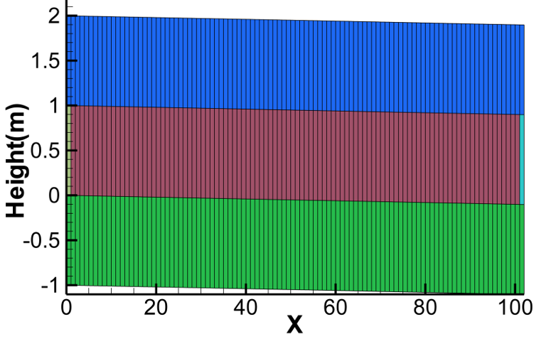
Here the effect of periodical variation of sea level due to tides to an adjacent confined aquifer was simulated and the simulation results were compared with analytical solutions. The following expressions formalize the analytical solution for the water level fluctuations in the confined aquifer due to the tidal effect.

\[w\left( t,x \right) = a \bullet exp\left( - \text{mx} \right)\cos\left( \sigma\text{t} - \text{mx} \right)\]

with

\[\begin{matrix} \sigma = \frac{2\pi}{T} \\ m = \sqrt{\frac{\sigma\text{S}}{\left( 2\text{Kb} \right)}} \\ S = \rho_{w}\phi\text{gb}\left( C_{f} + C_{r} \right) \\ \end{matrix}\]

where, \(w\left( t,x \right)\) is the fluctuation around the mean sea level [m], \(a\) is the tidal amplitude [m], \(x\) is the distance from the coast [m], \(t\) is the time [s], \(T\) is the cycle time [s], \(S\) is the storage coefficient [-], \(K\) is the hydraulic conductivity [m/s], \(b\) is the thickness of confined aquifer [m], \(\phi\) is the effective porosity [-], \(\rho_{w}\) is the liquid density [kg/m³], \(g\) is gravitational acceleration [m/s²], \(C_{f}\) is the compressibility of liquid [1/Pa], \(C_{r}\) is the compressibility of aquifer media [1/Pa]. Note that to obtain the water level fluctuation from the bottom of sea, is the mean sea level \(h\) [m] should be added to \(w\left( t,x \right)\).

Figure 3.18: Concept of the tidal movement in an aquifer (C-I-6)

Numerical model

Table 3.35: Specifications of the numerical model (C-I-6).
	Symbol	Units	Value
Total No. of grids	NNBLK	[-]	3417
No. of grids in X direction	NX	[-]	201
No. of grids in Y direction	NY	[-]	1
No. of grids in Z direction	NZ	[-]	17

Model parameters

Table 3.36: Fluid properties (C-I-6).
Property	Units	Value	Symbol
Aqueous phase density	[kg/m³]	998.2	\(\rho~w~\)
Aqueous phase compressibility	[1/Pa]	4.59×10^-5	\(C~f~\)
Aqueous phase viscosity	[Pa s]	1.002×10^-3	\(\mu\)
Coefficient of aqueous phase viscosity	[1/Pa]	0	\(C~\mu~\)

Table 3.37: Layer properties (C-I-6).
	Symbol	Units	Aquiclude	Confined Aquifer	Boundary	Sea
Density	\(\rho\)	[kg/m³]	2500	2500	2500	2500
Porosity	\(\varphi\)	[-]	0.2	0.2	1.0×10³⁰	1.0×10³⁰
Permeability	K	[m²]	0	1.0×10^-12	9.87×10³⁴	9.87×10³⁴
Compressibility ratio	C_r	[1/Pa]	1.02×10^-5	1.02×10^-5	1.02×10^-5	1.02×10^-5

Table 3.38: Parameters of tidal fluctuation calculation (C-I-6).
	Symbol	Units	Value
Initial water level	h₀	[m]	-5
Tidal amplitude	a	[m]	1
Periodical cycle	T	[s]	86400
Thickness of the confine aquifer	b	[m]	5
Mean sea level position	h	[m]	-5

Results

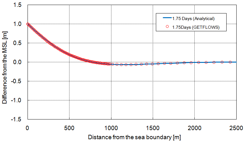
Fig: Comparison of analytical and numerical results for the water level fluctuation in the aquifer from sea boundary (C-I-6)

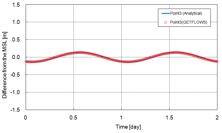
Fig: Residual water level fluctuations from mean sea level at different points with time (C-I-6)

Error estimation

The root mean square error (RMSE) was used to compare the analytical results and the results of GETFLOWS simulation. The RMSE is computed with:

\[RMSE = \sqrt{\frac{1}{N}\sum_{i = 1}^{N}\left( A_{i} - N_{i} \right)^{2}}\]

Table 3.39: RMSE of water level at different time intervals (C-I-6).
Elapsed time [day]	Comparison interval [m]	No. of comparison points	RMSE [m]
0.5	[0,2500]	120	5.019×10-3
1	[0,2500]	120	5.655×10-3
1.25	[0,2500]	120	3.852×10-3
1.75	[0,2500]	120	2.979×10-3

Table 3.40: RMSE of water levels at three locations (C-I-6).
Location	Comparison interval [day]	No. of comparison points	RMSE [m]
Point1	[0,2]	201	1.193×10-4
Point2	[0,2]	201	5.709×10-3
Point3	[0,2]	201	4.378×10-3

C-I-7: Unsaturated zone capillary pressure curves

Summary

Table 3.41: Test properties (C-I-7).
Test categoty	`[o]` Analytical solution, `[_]` Benchmark, `[_]` Test data
Fluid system	`[o]` isothermal, `[_]` non-isothermal
	`[o]` water, `[o]` gas (air), `[_]` NAPL, `[_]` species composition
Type of analysis	water- air 2 phase flow
Dimension	`[o]` 1-dimension, `[_]` 2-dimension, `[_]` 3-dimension
Entry list	`ci17.dat`
References
Compared to	Excel file
GETFLOWS base input	base-input
GETFLOWS card input	[card-input][CI7_card]

Description

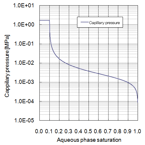
A uniform unconfined aquifer was considered in which the water table lied 100 m below the ground surface. Effective water saturation in the unsaturated zone was theoretically calculated and compared with the simulator results. GETFLOWS numerical calculation in this simulation was based on water – air two phase fluid system. However in the present calculation the movement of air was neglected. Here, the Van–Genuchten expression was used to calculate the water saturation and capillary pressure of the unsaturated area in GETFLOWS. The effective water saturation takes for following expression:

\[S_{e} = \frac{1}{\left( 1 + \left( \alpha\left| h_{c} \right| \right)^{n} \right)^{m}}\]

Expressed as a function of the saturation, the capillary head takes for form:

\[h_{c} = \frac{1}{\alpha}\left( \frac{1}{{S_{e}}^{1/m}} - 1 \right)^{1/n}\]

In these expressions, \(S_{e}\) is the effective saturation [-], \(h_{c}\) is the capillary head [m], \(\alpha\) is a parameter that depends on the reciprocal pressure of the non-wetting phase (air) [1/Pa], \(n\) and \(m\) are the Van-Genuchten parameters with \(n\) representing the uniformity of porous media specific to the soil type (high uniformity if \(n\) is large) and \(m = 1 - 1/n\).

Numerical model

Table 3.42: Specifications of the numerical model (C-I-7).
	Symbol	Units	Value
Total No. of grids	NNBLK	[-]	203
No. of grids in X direction	NX	[-]	1
No. of grids in Y direction	NY	[-]	1
No. of grids in Z direction	NZ	[-]	203
Column height	L	[m]	100
Cross sectional area of the column	A	[m²]	1
Gravitational acceleration	g	[m/s²]	9.80665

Model parameters

Table 3.43: Fluid properties (C-I-7).
	Symbol	Units	Value
Aqueous phase density	\(\rho_{w}\)	[kg/m³]	1000.0
Gas phase density	\(\rho_{g}\)	[kg/m³]	0.0
Aqueous phase compressibility	\(C_f\)	[1/Pa]	0
Aqueous phase viscosity	\(\mu\)	[Pa s]	1.002×10^-3
Coefficient of aqueous phase viscosity	\(C_\mu\)	[1/Pa]	0
Irreducible saturation	\(S_{irr}\)	[ ]	0.01

Table 3.44: Layer properties (C-I-7).
	Symbol	Units	Atmosphere	Surface	Underground	Upstream
Density	\(\rho\)	[kg/m³]	2500	2500	2500	2500
Porosity	\(\varphi\)	[-]	1.0×10³⁰	1.0×10³⁰	0.2	1.0×10³⁰
Permeability	\(K\)	[m²]	9.87×10^-6	9.87×10^-6	9.87×10^-13	9.87×10^-13
Compressibility ratio	\(C_r\)	[1/Pa]	0.0	0.0	0.0	0.0

Relative permeability Curve (C-I-7) capillary pressure curves (C-I-7)

Fig: Multiphase parameters - Relative permeability and capillary pressure curves (C-I-7){#fig:ci7pc}

Note that the hydrostatic condition is activated from the layer 203.

Results

Error estimation

The root mean square error (RMSE) was used to compare the analytical results and the results of GETFLOWS simulation. The RMSE is computed with:

\(RMSE = \sqrt{\frac{1}{N}\sum_{i = 1}^{N}\left( A_{i} - N_{i} \right)^{2}}\).

Table 3.45: RMSE estimation for analytical and numerical solutions(C-I-7).
Compared depth [m]	No of points	RMSE [m]
[0,100]	201	4.275×10-3

C-I-8: Calculation of a benchmark of multiphase flow simulator – TOUGH2

Summary

Table 3.46: Test properties (C-I-8).
Test category	`[_]` Analytical solution, `[_]` Benchmark, `[_]` Test data
Fluid system	`[o]` Isothermal, `[_]` non-isothermal
	`[o]` water, `[o]` gas (air), `[_]` NAPL, `[_]` species composition
Type of analysis	water-gas 2 phase flow
Dimension	`[_]` 1-dimension, `[o]` 2-dimension, `[_]` 3-dimension
Entry list	`ci18.dat`
References	Thunvik, R., 1987. Calculation on HYDROCOIN level 1 using the GWHRT flow model, SKB Technical Report 87-03.
GETFLOWS base input	base-input
GETFLOWS card input	[card-input][CI8_card]

Description

Groundwater flow in a porous media with heterogeneous permeability was simulated by GETFLOWS and general purpose multiphase flow simulator TOUGH2. Two dimensional heterogeneous porous media which is sandwiched between impermeable layers as shown in Figure 31 is considered for the simulation. Initially the system was kept at unsaturated condition then water was injected and allowed to flow through the media replacing the air. Transient process results were checked at two different points and compared as show in following figures

Figure 3.22: Heterogeneous soil system (C-I-8)

Numerical model

Table 3.47: Specifications of the numerical model (C-I-8).
	Symbol	Units	Value
Total No. grids	NNBLK	[-]	286
No. of grids in X direction	NX	[-]	22
No. of grids in Y direction	NY	[-]	1
No. of grids in Z direction	NZ	[-]	13
L	L	[m]	20
H	H	[m]	10
A	A	[m]	3
B	B	[m]	1
Gravitational acceleration	g	[m/s²]	9.80665

Analysis condition

Inflow pressure boundary condition - 0.297436 [MPa]

Inflow pressure boundary condition - 0.101303 [MPa]

Table 3.48: Fluid properties (C-I-8).
Property	Symbol	Units	Value
Aqueous phase density	\(\rho\)_w	[kg/m³]	998.2
Gas phase density	\(\rho\)_g	[kg/m³]	0.0
Aqueous phase compressibility	C_f	[1/Pa]	4.5×10^-5
Aqueous phase viscosity	\(\mu\)_w	[Pa s]	1.002×10^-3
Coefficient of aqueous phase viscosity	C_\(\mu\)	[1/Pa]	1.0×10^-5

Table 3.49: Layer properties (C-I-8).
Property	Symbol	Units	Atmosphere	Surface	Permeable Stratum	Impervious Stratum	Injection Point	Outflow Boundary
Density	\(\rho\)	[kg/m³]	2500	2500	2500	2500	2500	2500
Porosity	\(\phi\)	[-]	1.0×10³⁰	1.0×10³⁰	0.2	1.0×10³⁰	1.0×10³⁰	1.0×10³⁰
Permeability	K	[m²]	9.87×10^-6	0	1.00×10^-11	0	1.00×10^-11	1.00×10^-11
Compressibility ratio	\(C_r\)	[1/Pa]	1.02×10^-5	1.02×10^-5	1.02×10^-5	1.02×10^-5	1.02×10^-5	1.02×10^-5

Multiphase parameters - Relative permeability and capillary pressure curves (C-I-8){#tbl:ci8pc}
Relative permeability curves	Capillary pressure curves

Results

Table 3.50: Comparison of Comparison of numerical results for the water saturation between GETFLOWS and TOUGH2 (C-I-8).
	GETFLOWS	TOUGH2	Legend
0.05 days
0.1 days
0.3 days
0.5 days

Error estimation

The root mean square error (RMSE) was used to compare the analytical results and the results of GETFLOWS simulation. The RMSE is computed with:

\(RMSE = \sqrt{\frac{1}{N}\sum_{i = 1}^{N}\left( A_{i} - N_{i} \right)^{2}}\).

Table 3.51: RMSE error analysis (C-I-8).
Location	Time duration [s]	Nb of points for comparison	RMSE Pressure [MPa]	RMSE Saturation [-]
Point1	0-86400	3876	9.8636×10-4	5.8975×10-3
Point2	0-86400	3876	5.4307×10-4	6.5300×10-3

Category II

C-II-1: Solute transport in one dimensional confined aquifer (work-in-progress)

Summary

Table 4.1: Test properties (C-II-1).
Test classification	`[o]` Analytical solution, `[_]` Benchmark, `[_]` Test data
Fluid system	`[o]` Isothermal, `[_]` non-isothermal
	`[o]` water, `[o]` gas (air), `[_]` NAPL, `[_]` species composition
Type of analysis	water- gas 2 phase flow, transport
Dimension	`[o]`1-dimension, `[_]`2-dimension, `[_]`3-dimension
Entry list	`ci18.dat`
References	Charles Fitts, Groundwater science, Academic Press 2002 (p.381), Ogata and Banks (1961)
Compared to	Excel file
GETFLOWS base input	[base-input][CII1_base]
GETFLOWS card input	[card-input][CII1_card]

Outline

This case is to simulate the solute transport in one dimension when chemical substance with assigned concentration is continuously injected at the source point (as Fig.1 shows below). The solute transport can be described with one dimensional convection-dispersion equation as follows.

\[- v\frac{\partial C}{\partial x} + D\frac{\partial^{2}C}{\partial x^{2}} = \ \frac{\partial C}{\partial t}\]

where \(D = D_0\varphi/\tau+ \alpha v\), \(D_0\) is the diffusion coefficient obtained by experiment to describe molecular diffusion, and D is the coefficient to describe hydrodynamic dispersion which also includes mechanical dispersion(\(\alpha v\)). The meaning of each parameter concerned is given in table1.

The rigorous solution of the equation is

\[C\left( x,t \right) = \ \frac{C_{0}}{2}\lbrack erfc\left( \frac{x - vt}{2\sqrt{\text{Dt}}} \right) + erfc(\frac{x + vt}{2\sqrt{\text{Dt}}})exp(\frac{\text{vx}}{D})\rbrack\]

\[\text{erfc}\left( x \right) = 1 - \operatorname{erf}\left( x \right) = 1 - \frac{2}{\sqrt{\pi}}\int_{0}^{x}{e^{- \varepsilon^{2}}\text{d}\varepsilon}\]

With the boundary condition of

\(C\left( x = 0 \right) = C_{0}\)
\(C\left( x = L \right) = C_{L}\)

Description (Assumptions and Limitations)

The problem is depicted in Figure {Fig. 4.1}. A fluid flow steady state is established. The solute transport simulation is executed assuming an initial situation with concentration of 0.01 at inlet point (upstream) and 0 at outlet point (downstream). The dispersion length (\(\alpha\)) is assumed to be 0.03. The inlet and outlet concentration remains the same as initial value for the entire simulation.

Figure 4.1: Schematic drawing of the geometry and boundary conditions for the 1-D conservative solute transport

Table 4.2: Input Parameters for 1-D solute transport Problem.
Parameter	Symbol	Units	Value
Fluid actual Velocity	v	m/s	0.019128
Flow Path Length	L	m	10
Diffusion Coefficient	D₀	m²/s	0.0005
Porosity	\(\varphi\)	[-]	0.5
Tortuosity	\(\tau\)	[-]	1
Dispersion Length	\(\alpha\)	m	0.03
Pressure	P	Mpa	0.1033
Boundary Conditions	At x = 0	C₀ = 0.01
	At x = 10	C_L = 0

Numerical Model

10m length of the column was divided into 1.0m equal size grid mesh, including 2 grids for boundaries. Total number of grids assigned for this case is 12 as shown in Fig. 2. Fixed pressure head boundary conditions were are assigned at the ends of the column to maintain steady state flow rate through the porous media.

One dimensional numerical model for porous media {#fig:F29b}

Table 4.3: Specifications of the numerical model
	Symbol	Units	Value
Total NO. of grids	NNBLK	[-]	48
NO. of grids in X direction	NX	[-]	12
NO. of grids in Y direction	NY	[-]	1
NO. of grids in Z direction	NZ	[-]	4
Width of the column	W	[m]	1
Length of the column	L	[m]	10
water depth	h	[m]	1

Table 4.4: Boundary condition
Boundary Conditions at \(NX= 1\)	\(C_0 = 0.01\)	\(P_0 = 2.1033\)
Boundary Conditions at \(NX= 12\)	\(C_L = 0\)	\(P_L= 0.1033\)

Analysis condition

Table 4.5: Fluid properties
	Symbol	Units	Value
Aqueous phase density	\(\rho\)_w	[Kg/m³	] 998.2
Aqueous phase compressibility	C_f	[1/Pa]	0
Aqueous phase viscosity	\(\mu\)	[Pa.s]	1.002*10^-3
Aqueous phase viscosity coefficient	C_\(\mu\)	[1/Pa]	0

Table 4.6: Layer properties
	Symbol	Units	Atmosphere	Surface	Impervious Stratum	Permeable Stratum
Density	\(\rho\)	[Kg/m³]	2500	2500	2500	2500
Porosity	\(\varphi\)	[-]	1.0d30	1.0d30	1.0d30	0.5
Permeability	Kr	[md]	1.0d30	1.0d30	0.0d30	1.0d5
Compressibility	Cr	[1/Pa]	0	0	0	0

Results

Figure Comparative analysis – GETFLOWS vs. Analytical Solution by EXCEL

Error estimation

The root mean square error (RMSE) was used to compare the analytical results and the results of GETFLOWS simulation. The RMSE is computed with:

\(RMSE = \sqrt{\frac{1}{N}\sum_{i = 1}^{N}\left( A_{i} - N_{i} \right)^{2}}\).

Table 4.7: Estimated error comparison for GETFLOWS and EXCEL.
Distance from upstream end [m]	Number of points	RMSE
1	100	0.0011319
3	100	0.0021811
5	100	0.0029911
9	120	0.0039458

References

Ogata, A. and R. B. Banks, A solution of the partial differential equation of longitudinal dispersion in porous media, U.S. Geological Survey Professional Paper 411-A (1961)

Tests classification

Table 6.1: Features validated by each test case.
Fluid system	V&V test case
Fluid phase
F-1: Aqueous phase
F-2: Gas phase	C-I-1, C-I-2, C-I-3, C-I-4,C-I-5,C-I-6, C-I-7, C-I-7mod, C-I-8
F-3: Non-aqueous phase liquid (NAPL)	C-I-1, C-I-2, C-I-4, C-I-6, C-I-7, C-I-mod, C-I-8
Fluid characteristics
F-4: Density
F-5: Viscosity	C-I-1, C-I-2, C-I-3, C-I-4,C-I-5,C-I-6, C-I-7, C-I-7mod, C-I-8
F-6: Pressure dependence	C-I-1, C-I-2, C-I-3, C-I-4,C-I-5,C-I-6, C-I-7, C-I-7mod, C-I-8
F-7: Temperature dependence	C-I-2, C-I-5, C-I-6, C-I-7, C-I-8
F-8: Super critical state
Surface flow	V&V test case
Flow characteristics
R-1: Uniform flow	C-I-1
R-2: Non-uniform flow	C-I-2
R-3: Unsteady flow	C-I-2
R-4: Infiltration
R-5: Discharge
Open channel flow
Mean velocity formula
R-6: Manning’s equation	C-I-1,2
R-7: Chezzy’s formula
Solving the equation of motion
R-8: Dynamic Wave
R-9: Diffusion wave approximation
R-10: Linearized diffusion wave approximation	C-I-1,2
R-11: Motion wave approximation
Runoff model
R-12: Storage function method
R-13: Tank model
R-14: Distributed model	C-I-1,2
Land use characteristics
R-15: Rainfall distribution
R-16: Temporal variation of rainfall
R-17: Snow cover . snow melting
R-18: Evapotranspiration
R-19: Sea level change	C-I-6, C-I-7
R-20: Land use
R-22: Canopy interception
R-23: Litter interception	C-I-1,2
Surface flow parameters
R-24: Equivalent roughness coefficient
Man-made structures
R-25: Sluice gate-sluice
R-26: Weir
R-27: Dam
R-28: Storm water infiltration facilities
R-29: Artificial recharge facilities
Solute transport	V&V test case
Conservative transport process
T-1: Advection
T-2: Mechanical dispersion
T-3: Molecular diffusion
T-4: Multi-component
Inter phase mass transfer
T-5 : Adsorption (Vapour→Solid )
T-6 : Adsorption (Liquid →Solid )
T-7 : Desorption (Solid → vapour)
T-8 : Desorption (Solid → Liquid )
T-9 : Volatilization
T-10: Condensation
Suction
Isothermal adsorption equilibrium
T-11: Linear(Retardation)
T-12: Langmuir
T-13: Freudlich
T-14: Adsorption kinetics
Chemical reaction
T-15: Ion exchange
T-16: Substitution / Hydrolysis
T-17: Dissolution (Vapour → Aqueous)
T-18: Dissolution(Non-aqueous phase → Aqueous phase)
T-19: Dissolution (Solid → Aqueous)
T-20: Precipitation
T-21: Oxidation／Reduction
T-22: Acid-base reaction
T-23: Complex formation
T-24: Microbial degradation
T-25: Radioactive decay
Response format
T-26: Zero order reaction
T-27: 1st order reaction
T-28: 2nd order reaction
T-29: Chain reaction
Solute transport parameters
T-30: Porosity
Dispersion length
T-31: Isotropy
T-32: 2D anisotropy
T-33: 3D anisotropy
T-34: Homogeneous
T-35: Heterogeneity
T-36: Scale dependency
Diffusion coefficient
T-37: Homogeneous
T-38: Heterogeneity
T-39: Multi-component
Retardation factor
T-40: Homogeneous
T-41: Heterogeneity
T-42: Tortuosity
T-43: Reaction rate constant
T-44: Henry’s Constant
T-45: Half-life
Sink/Source
Point sources (Wells)
T-46: Constant flow/concentration injection
T-47: Variable flow/concentration injection
T-48: Groundwater withdrawal
T-49: Radiation source(Infiltration trench)
T-50: Horizontal plane source(Farms, Reclaimed site)
T-51: plant uptake
Output	V&V test case
Echo back
O-1: Echo of the input	C-I-1, C-I-2, C-I-3, C-I-4,C-I-5,C-I-6, C-I-7, C-I-7mod, C-I-8
Results output (format)
O-2: Binary format	C-I-1, C-I-2, C-I-3, C-I-4,C-I-5,C-I-6, C-I-7, C-I-7mod, C-I-8
O-3: ASCII format	C-I-1, C-I-2, C-I-3, C-I-4,C-I-5,C-I-6, C-I-7, C-I-7mod, C-I-8
O-4: Spatial distribution	C-I-1, C-I-2, C-I-3, C-I-4,C-I-5,C-I-6, C-I-7, C-I-7mod, C-I-8
O-5: Time series	C-I-1, C-I-2, C-I-3, C-I-4,C-I-5,C-I-6, C-I-7, C-I-7mod, C-I-8
O-6: Screen display (text)	C-I-1, C-I-2, C-I-3, C-I-4,C-I-5,C-I-6, C-I-7, C-I-7mod, C-I-8
O-7: Screen display (graph)
O-8: Image file
Results output (type)
O-9: Pressure	C-I-1, C-I-2, C-I-3, C-I-4,C-I-5,C-I-6, C-I-7, C-I-7mod, C-I-8
O-10: Potential	C-I-1, C-I-2, C-I-3, C-I-4,C-I-5,C-I-6, C-I-7, C-I-7mod, C-I-8
O-11: Saturation factor	C-I-1, C-I-2, C-I-3, C-I-4,C-I-5,C-I-6, C-I-7, C-I-7mod, C-I-8
O-12: Pressure variation
O-13: Saturation variation
O-14: Interstitial flux	C-I-1, C-I-2, C-I-3, C-I-4,C-I-5,C-I-6, C-I-7, C-I-7mod, C-I-8
O-15: Infiltration flux	C-I-4
O-16: Evapotranspiration flux
O-17: Boundary flux
O-18: Flow rate / velocity	C-I-1, C-I-2, C-I-3, C-I-4,C-I-5,C-I-6, C-I-7, C-I-7mod, C-I-8
O-19: Stream lines- Path of particles (image)
O-20: Mass balance
Calculated information output
O-21: Iteration progress	C-I-1, C-I-2, C-I-3, C-I-4,C-I-5,C-I-6, C-I-7, C-I-7mod, C-I-8
O-22: Iteration error	C-I-1, C-I-2, C-I-3, C-I-4,C-I-5,C-I-6, C-I-7, C-I-7mod, C-I-8
O-23: Mass balance error
O-24: CPU time
O-25: memory allocation
Subsurface fluid flow	V&V test case
Flow characteristics
G-1: Single phase flow	C-I-3, C-I-4, C-I-5, C-I-6, C-I-7, C-I-8
G-2: Two phase flow	C-I-8
G-3: Multiphase flow
G-4: Water Vapour
G-4: Brine(Density flow)
G-6: Darcy’s flow	C-I-3, C-I-4, C-I-5, C-I-6, C-I-7, C-I-8
G-7: Non-Darcy’s flow
Hydrological characteristics of the media
G-8: Porous media	C-I-3, C-I-4, C-I-5, C-I-6, C-I-7
G-9: Discrete fracture
G-10: Dual porosity model
G-11: Homogeneous hydraulic properties	C-I-3, C-I-4, C-I-5
G-12: Heterogeneous hydraulic properties	C-I-6, C-I-7, C-I-8
G-13: Anisotropic hydraulic properties
G-14: Compressible soil	C-I-5, C-I-6, C-I-7, C-I-8
G-15: Swelling
G-16: Shrinking
G-17: Dipping layer
G-18: Multi-layer type	C-I-6, C-I-7, C-I-8
Media parameters
G-19: Porosity	C-I-3, C-I-4, C-I-5, C-I-6, C-I-7, C-I-8
G-20: Porosity variation
G-21: Permeability	C-I-3, C-I-4, C-I-5, C-I-6, C-I-7, C-I-8
G-22: Permeability variation
G-23: Compression ratio	C-I-5, C-I-6, C-I-7
G-24: Residual saturation
Saturation vs Capillary pressure(suction)
G-25: Model selection
G-26: Tabular input (optional)	C-I-8
G-27: Hysteresis
Saturation factor vs Relative permeability
(Unsaturated hydraulic conductivity)
G-28: Model selection
G-29: Tabular input (optional)
G-30: Hysteresis
G-31: Three phase relative permeability model	C-I-8
Fluid process
G-32: Infiltration of surface water
G-33: Evapotranspiration	C-I-4
G-34: Formation of capillary zone
Sink/Source
Point sources (Wells)
G-35: Constant flow	C-I-5
G-36: Variable flow
G-37: Constant pressure	C-I-6, C-I-7, C-I-8
G-38: Well loss
G-39: Grid-radius compensation	C-I-5
G-40: Well-bore storage
G-41: Multilayer completion	C-I-5
Radiation source
G-42: Constant flow
G-43: Variable flow
G-44: Constant pressure	C-I-3, C-I-4, C-I-8
Heat transport	V&V test case
Heat transport mechanism
H-1: Advection
H-2: Heat conduction
H-3: Thermal dispersion
H-4: Solid phase－liquid thermal diffusion
H-5: Radiation
H-6: Phase-change
H-7: Heat exchange between phases
Point sources (Wells)
H-8: Heat generation
Heat transport parameters
H-9: Porosity
Thermal dispersion coefficient
H-10: Isotropy
H-11: Anisotropy
H-12: Homogeneous
H-13: Heterogeneity
Solid thermal conductivity
H-14: Homogeneous
H-15: Heterogeneity
Sink/Source
H-16: Constant flow-temperature injection
H-17: Variable flow-temperature injection
H-18: Groundwater withdrawal
H-19: Radiation source
H-20: Horizontal plane source
Sediment transport	V&V test case
Sediment transport process
S-1: Bed load
S-2: Suspended sediment
S-3: Slope failure
S-4: Topographic change
S-5: Spread terrain
Sediment transport parameters
S-6: Particle size distribution
S-7: Particle density
S-8: subjugation coefficient
Numerical solution - Solver	V&V test case
Spatial orientation
N-1: 1-Dimensional horizontal	C-I-1, C-I-2, C-I-3
N-2: 1-Dimensional vertical	C-I-3, C-I-4
N-3: 2-Dimensional horizontal
N-4: 2-Dimensional vertical	C-I-6, C-I-7, C-I-8
N-5: 2-Dimensional radial
N-6: Fully 3-dimensional	C-I-5
N-7: 3-Dimensional cylindrical
N-8: 3-Dimensional radial
Space discretization
N-9 : No discretization
N-10: Uniform grids	C-I-1, C-I-2, C-I-3, C-I-4, C-I-8
N-11: Variable grid spacing	C-I-5, C-I-6, C-I-7
N-12: Moving grid (Node relocation)
N-13: Local Grid Refinement (LGR)
Grid formation
N-14: 1-dimensional linear
N-15: 1-dimensional nonlinear
N-16: 2-dimensional triangular
N-17: 2-dimensional nonlinear triangular
N-18: 2-dimensional rectangular
N-19: 2-dimensional square
N-20: 2-dimensional quadrilateral
N-21: 2-dimensional nonlinear quadrilateral
N-22: 2-dimensional polygon
N-23: 2-dimensional cylindrical
N-24: 3-dimensional cube
N-25: 3-dimensional rectangular
N-26: 3-dimesional hexahedral	C-I-1, C-I-2, C-I-3, C-I-4,C-I-5,C-I-6, C-I-7, C-I-7mod, C-I-8
N-27: 3-dimensional tetrahedron
N-28: 3-dimensional spherical
Numerical solution
N-29: Finite difference method
N-30: Integral finite difference method	C-I-1, C-I-2, C-I-3, C-I-4,C-I-5,C-I-6, C-I-7, C-I-7mod, C-I-8
N-31: Finite element method
N-32: Particle tracking method
Time discretization
N-33: Explicit method
N-34: Fully implicit method	C-I-1, C-I-2, C-I-3, C-I-4,C-I-5,C-I-6, C-I-7, C-I-7mod, C-I-8
N-35: Crank-Nicholson low
Time Stepping Scheme
N-36: Fixed time step	C-I-2
N-37: Variable time step	C-I-1, C-I-3, C-I-4,C-I-5,C-I-6, C-I-7, C-I-7mod, C-I-8
Nonlinear solution
N-38: Picard’s successive iteration method
N-39: Newton-Raphson low	C-I-1, C-I-2, C-I-3, C-I-4,C-I-5,C-I-6, C-I-7, C-I-7mod, C-I-8
Matrix Solver
N-40: Iteration	C-I-1, C-I-2, C-I-3, C-I-4,C-I-5,C-I-6, C-I-7, C-I-7mod, C-I-8
N-41: Direct method
N-42: Successive locking process (SLP)

GETFLOWS verification and validation manual (V&V)

V&V category I & II

Geosphere Environmental Technology Corp. (GET Corp.)

NCO Kanda Awajicho-Build. 3F

2-1 Kanda Awajicho, Chiyoda-ku, Tokyo 101-0063, Japan

Phone: 03-5283-5825 (representative), http://www.getc.co.jp/english

@Copyright Geoshpere environmental technology Corp.

1999. Mathematics of Geo-Hydrological Cycles, University of Tokyo Press (in Japanese). Springer.

Tosaka, H. 2007. “Mathematics of Geo-Hydrological Cycles, 86-89, University of Tokyo Press. (In Japanese).”

When we mention “Verification”, we mean that we solve the independently conducted benchmark questions and evaluate the properties in function and operation. In addition, we test the built-in algorithm and the internal data processing; as a result we can demonstrate the consistency, integrity and reliability in the codes regarding the design basis. When we mention “Validation”, we mean that we confirm the relevance of the theoretic foundation and the modeling of the codes writing the behavior of real system through comparison between independently observed groundwater system response and the calculation result. Regarding the difference between the two notions, one intends to confirm the closed system without considering the uncertainty and the other intends to confirm the open system included the uncertainty.

Source: Verification and Validation in the universal value simulator analyzing the water and material circulation, Yasuhiro Tawara, Koji Yamashita and others, summary of the speech in the conference of Japanese Association of Groundwater Hydrology, spring 2010.↩︎