GETFLOWS Theory Manual
Geosphere Environmental Technology Corp.
v1.0.0 – 2021/05/31
About
This document provides details about the fundamental theory and numerical analysis used in the 3D general-purpose numerical flow simulator GETFLOWS, which is used for analyzing water flow in the biosphere on land (the geosphere) and the transport behavior of accompanying matter and heat.
Water transported in the water cycle is both a valuable resource that must be preserved to ensure the advancement of human civilization and, at the same time, the cause of various disasters. A large portion of the history of humankind involves battles with nature, and water has played a major role in these battles. Water is also a global issue for the coming century. Specifically, numerous problems must be tackled, including the development, management, and conservation of water resources such as rivers, lakes, dams, and groundwater; evaluation of and measures against changes in the water environment and water pollution; and prediction of and measures against large-scale natural disasters, such as floods, landslides, and mudflows. To address these problems, it is necessary to examine and survey the natural environment both globally and locally, to perform quantitative and comprehensive evaluation of the data, and to implement relevant administrative policies (on the environment, disaster prevention facilities, and so on).
In recent years, the increased resolution of global terrain information obtained from information-gathering satellites has allowed all interested people to obtain graphical information in the form of stunning images and positioning information for tasks such as car navigation. This means that it has become possible to observe the “shape of fields” near the ground surface. In addition, it has become possible to observe the dynamic movement of clouds in the atmosphere, and the accuracy of weather forecasting has been improved dramatically.
However, nature is enormous in terms of both space and time. It is both complex and obscure. There are many phenomena that cannot be predicted, even when observed, and many for which it is unclear what countermeasures should be taken. Furthermore, there are still many phenomena that cannot be observed at all (such as subsurface processes). For this reason, no amount of debate by experts and citizens in regard to environmental problems and other issues can settle which events will come to pass and which ones will not.
The simulation system introduced here provides a computer-based representation of fields in nature on land, together with fluid flows that take place in those fields. It makes forecasts about the results of interplay between processes occurring in various and extensive natural systems, which cannot be intuitively forecast by humans. The simulation system uses as few arbitrary manual settings as possible and employs various schemes to represent nature as naturally as possible. However, it is frequently the case that incomplete information about nature is available, and so there necessarily remain some parameters that must be estimated. Often, expertise is needed to evaluate the accuracy of the data, the suitability of the boundary and initial conditions, and the reliability of the analysis results.
This software originally targeted experts, with the aim of responding to the demand for reliable information about the effects of administrative policies pertaining to large-scale operations to be undertaken by countries and self-governing bodies. Therefore, a manual was not previously prepared for the fundamental theories. For this version, we have compiled this volume in the hope that it will serve as a reference to researchers, technicians, and students in this field. Although the manual is still incomplete, we plan to make gradual amendments as necessary.
We sincerely hope that the reader will find this manual useful.
Development history and current status of GETFLOWS
GETFLOWS (GEneral purpose Terrestrial fluid-FLOW Simulator) is a 3D general-purpose numerical simulator for analyzing fluid flows on land together with the transport behavior of associated matter and heat. It was developed between the mid-1980s and 1990s (Tosaka 1996). The basic technique of 3D three-phase oil layer analysis (developed by Tosaka at Japan Oil Engineering Co., Ltd., in the 1980s) was implemented in a completely overhauled form as a general-purpose simulator for groundwater analysis. As an example of its use, in the 1990s, the technique was applied to the evaluation of the impact of the aquatic environment on water sealing design and excavation operations for underground oil storage facilities by Yamaishi et al. (1997), in which surface flows were completely coupled. Furthermore, a version for simulation of heat circulation in drainage basins was developed at the end of the 1990s.
In 2000, Geosphere Environmental Technology Corp. was established as a university venture for performing third-party environmental and disaster evaluations, based primarily on GETFLOWS models, and the simulator itself was transferred to the corporation together with all related technologies.
Since then, the management, sale, maintenance, and development of the simulator (such as the parallelization of the simulator, extension of its capabilities, writing of manuals, and development of graphical tools) has been performed internally. There have been more than 500 scenarios considered during the past 10 years where GETFLOWS has been applied, encompassing various fields, such as water resources, environment, pollution, natural disasters and radioactive waste processing.
The program was originally written in FORTRAN 77, but much of it has since been rewritten in FORTRAN 90 and 95.
Introduction
The Geosphere System
Fig. 1.1 shows a cross-sectional view of land, which serves as a platform for all human activity. The figure shows the land area (ground surface), above which is the atmosphere (atmospheric boundary layer). Under the surface, there is the lithosphere, and to the side there is the hydrosphere (oceans). In recent years, these fields, which are intimately related to human civilization, have come to be collectively referred to as “the geosphere.” The term geosphere is used below in this sense.
The radiant energy arriving from the sun and the associated great water cycle are the strongest factors that promote and, at the same time, regulate the activities of humans, flora, and fauna in the geosphere. Solids such as soils and rocks form a relatively static field, whereas fluids such as water and atmosphere (air) move dynamically, forming a field where various hydrogeological processes (interactions between fluids and solids) take place.

In recent years, it has become possible to predict global climate changes by using climate models, to predict the tracks of typhoons, and to make weekly weather forecasts. In weather models, movements in the atmosphere and in the oceans are modeled on a grid with cell sizes on the order of 10 to 100 km; general models of the temperature, evapotranspiration, and other parameters pertaining to land are also incorporated into weather models. However, for the purpose of designing, building, and maintaining a biosphere simulation, it is necessary to take into account fields and phenomena that are much closer to the scale of human activity, such as those listed in Table 1.1 below.
| Atmosphere | Atmospheric flows at the atmospheric boundary layer, precipitation, solar radiation, long-wavelength radiation |
| Ground surface | Evapotranspiration, river flow, surface water retention such as in lakes, landslides, sediment movement, turbidity currents, and other solid–liquid mixed-phase flows |
| Lithosphere | Vertical water penetration from the ground surface, intrusion and discharge of air from gaps, groundwater flow in aquifer layers, flows of deep groundwater and heat, and saline density currents along the coast |
| Coastal hydrosphere | Outflows from river mouths, nutrient salt transport, fluctuations in tide level, and fluctuations in sea level |
There has been abundant conventional research concerning the above points in both the natural sciences (basic science, engineering, and agriculture) and the humanities. This research has been reflected to a large extent in policies implemented by countries and self-governing bodies.

What can it do? Analysis Options and Fields of Application
GETFLOWS was developed by unifying the results of existing research on land processes (such as river runoff analysis, groundwater analysis, and reservoir analysis) that was conducted in a broad range of academic fields. This research was combined for the purpose of contributing toward the safety of the biosphere and the preservation of the environment.
Analysis options
GETFLOWS is capable of modeling phenomena such as the ones listed in Table 1.2.
| Terrestrial fluid system composition \(\rightarrow\) Wat Analysis option \(\downarrow\) | er Air | NAP | L Mat | ter in Mat liquid phase | ter in Hea gaseous phase | t Sed | iment |
|---|---|---|---|---|---|---|---|
| Flood flows, inundation analysis | ✓ | ✓ | ✓ | ||||
| Water / air two-phase water circulation analysis | ✓ | ✓ | ✓ | ||||
| Saturated–unsaturated aquifer layer two-phase analysis | ✓ | ✓ | ✓ | ||||
| Water / air / NAPL multi-phase analysis | ✓ | ✓ | ✓ | ✓ | ✓ | ||
| Coupled analysis of the water and heat transport system | ✓ | ✓ | ✓ | ✓ | ✓ | ||
| Coupled analysis of fluctuations in water, sediment, and movable beds | ✓ | ✓ | ✓ | ✓ | |||
| Density flow analysis | ✓ | ✓ | ✓ | ||||
| Reactive substance shift analysis | ✓ | ✓ | ✓ | ||||
| Multi-component gas transport analysis | ✓ | ✓ | ✓ |
- Surface water flows
- Saturated-unsaturated groundwater flows
- Advective dispersion of solutes in aqueous and gaseous phases
- Two-phase flows (water + air, water + NAPL, air + NAPL)
- Three-phase flows (water + air + NAPL)
- Heat transfer (convection and diffusion)
- Heat exchange between liquid phases and surface solid phases
- Suspended sand, bed load transport
- Sedimentation and lifting of suspended sand
- Movable bed foundation containing mixed-size particles (sediment exchange layer)
- Dissolution and volatilization of NAPL into aqueous phases (mass transfer in NAPL / water phases)
- Dissolution and release of air in aqueous phases (mass transfer between gaseous and aqueous phases)
- Vaporization and condensation (mass transfer between gaseous and aqueous phases)
- Adsorption and desorption of solutes (mass transfer between liquid and solid phases)
- Disintegration and decay chains of radioactive nuclei
- Decay and generation of substances through chemical processes
Differences from conventional models
The features of GETFLOWS are summarized as follows.
Conventional river runoff analysis and groundwater analysis employ various high-level models. However, river runoff analysis, for instance, is based on an approximate model of groundwater flow and the groundwater model ignores surface conditions. The most prominent feature of GETFLOWS is its use of a model that represents the fluid flow of regions including from the atmospheric boundary layer to deep underground layers and from coastal zones to inland zones.
Conventional analysis focuses primarily on tracking the movement of water and ignores the movement of any air that may be present at the same time. This simulator takes into account multiple phases (air, water, non-aqueous phase liquid (NAPL), and solid) and multiple components (air, water, solutes, solids, and isotopes), which enables modeling nature as it is.
The simulator supports modeling that minimizes the setting of artificial boundary conditions.
GETFLOWS allows for flexible handling of liquid phases and the components of the terrestrial fluid flow system. The analysis options that are typically used in practical tasks are given in Table 1.2. All options are based on the analysis of a compressible water–air two-phase fluid, to which NAPL phases, materials, heat, and bed load transport are added according to the settings of the target terrestrial fluid flow system. Integrated analysis is performed by taking into account the interactions among these components.
Fields of Application
The fields to which GETFLOWS has been successfully applied to date are listed in Table 1.3.
| Category | Purpose | Analysis details |
|---|---|---|
| Integrated water management for drainage basins | Development and management of water resources | Simulation of water circulation in drainage basins, quantitative evaluation of the flooding suppression effect of dam construction, evaluation of the effects of forests, evaluation of the amount of groundwater resources, evaluation of the aquatic environment in drainage basins |
| Policies regarding water damage in drainage basins | Hydrological outflow analysis, detailed inundation analysis, effects of dam construction, quantification of the effects of dams on flood control basins, river improvement and vegetation, policy comparison | |
| Water catchment area management | Functions of forests in water catchment areas, solute transport, sediment transport, water quality of mountain streams, dam sedimentation | |
| Environment in lake and coastal areas | Nutrient salt load transport by rivers from wide areas, lake eutrophication, evaluation of nutrient salt inflow load, and other phenomena in coastal areas and harbors | |
| Water utilization and decontamination policies | Irrigation water | Irrigation water resources, nitrate/nitrogen pollution |
| Groundwater utilization | Adjustment of groundwater utilization, planning of well water planning, effects of cultivation facilities | |
| Soil and groundwater contamination | Evaluation of the impact of solute contamination (heavy metals, inorganic salts), pollution with substances insoluble in water (volatile organic compounds, hydrocarbons from crude oil) | |
| Building / environment | Evaluation of the impact of surface and subsurface structures on the environment | Ground subsidence, obstruction of large-scale hydrological regimes by tunnels, bridges, underground pipes, underground arcades and stations |
| Ecosystems | Evaluation of habitat potential, water content in soil, heat analysis | |
| Policies regarding heat in urban environments | Heat islands, water-permeable pavements, design and evaluation of the effects of rainwater infiltration facilities, underground heat utilization | |
| Waste disposal | Disposal of radioactive waste | Transportation of nuclides by groundwater, chemical processes and gas transfer in artificial barriers, evaluation of the local and extended flow field for the construction, operation and closure of geological repositories, evaluation of long-term safety |
| Underground storage of CO2 | Diffusive leakage of injected or dissolved gas underground CO2 storage | |
| Waste disposal sites | Evaluation of the impact on the environment around disposal sites, evaluation of design safety, leachate policies, generation and diffusion of methane gas | |
| Energy | Hydropower | Evaluation of the flow regime of creeks, evaluation of hydropower potential, evaluation of dam flooding |
| Underground heat sources | Utilization of shallow underground heat, utilization of deep underground heat and hot springs | |
| Gas / oil resources | Evaluation of the safety of underground facilities for oil and gas storage, evaluation of reservoir characteristics, EOR | |
| Experiment analysis | Laboratory and field experiments | Experiments on evaporation, seepage and permeation, tracer experiments, adsorption experiments |
| Research | Analysis of water circulation in drainage basins | |
| Analysis of mass circulation in drainage basins | Tracking of stable isotopes, sea floor springs |
Input and Output Data and Basic Functions
Input and Output Data
The atmospheric conditions, terrain, and various human activities on the ground surface (such as land use, farming, and deforestation) can be represented in detail in the numerical model of the surface and subsurface areas, which are discretized by using a 3D mesh. By implementing a temporal evolution of these activities, we can easily reconstruct past states and predict future changes.
The primary input data necessary for running GETFLOWS are described in Table 1.4. These input data are categorized into (1) physical properties pertaining to the fluids and the substance composition that define the target terrestrial fluid system; (2) ground conditions, such as weather and land use; (3) structure of geological strata; and (4) human-related factors, such as water use and building construction. Hydrological observation data, such as river flow rates, groundwater levels, water quality, and water temperature, are not necessary as input data except in special cases (for instance, when used as boundary conditions). Such observation data can be compared with analysis results and used as field information to verify the model’s faithfulness.
Table 1.5 shows the numerical output obtained from the analysis. The numerical output of GETFLOWS consists of a primary output, produced for each grid element, and secondary output calculated from the primary output.
The primary output contains various quantities that obey conservation laws (such as phases and components constituting the fluid system), which are analyzed directly as numerical solutions. Output is produced for each fluid phase and components for all grid elements.
The secondary output consists of quantities obtained analytically from the primary variables. This includes the fluid potential (calculated from grid pressure) and liquid phase flux (calculated from water depth and fluid potential difference between grid elements). The flow velocity is output as quantities per unit time for each liquid phase at the interface between neighboring grid elements. The flow line trajectory and the residence time along the flow path are used for constructing a linearly interpolated flow velocity field and are calculated using flow-line tracing. Physical properties, read from an input file, and related parameters, calculated internally by the simulator, can be output to permit rigorous checking of the settings provided to the model.
| Input category | Data |
|---|---|
| Physical properties of fluids | Density, viscosity, compressibility, thermal conductivity, specific heat |
| Characteristics of chemical species | Molecular diffusion coefficient, half-life, maximum solution concentration, solubility, adsorption parameters, phase transition parameters (transition coefficient, area, etc.), saturated vapor pressure, Henry constant, molecular weight |
| Weather | Precipitation amount (rain and snow), atmospheric pressure, air temperature, possible duration of sunshine, solar irradiance, evapotranspiration, tide level |
| Terrain | Land area, sea area, river beds, lakes, dam lakes |
| Land use | Land use, equivalent roughness coefficient, vegetation / coverage |
| Geology | Surface soil, subsurface geology, absolute permeability, effective porosity, relative permeability, capillary pressure, compressibility, density, diffusion length, tortuosity, thermal conductivity, specific heat |
| Sediment | Grain size / mixing ratio, soil grain density, bed load transport parameters, suspended sand transport parameters, turbulent diffusion coefficient, maximum thickness of sediment exchange layer |
| Water use | Pumping wells (hole diameter, screen depth), irrigation water, irrigation channels / conduits, amounts of intake / drainage water |
| Use of artificial structures | Dams / sluices, sewerage treatment areas, water volume, pumping stations, rainwater storage and infiltration facilities, subsurface structures |
| Primary output | Secondary output calculated from the primary output |
|---|---|
| Pressure | Fluid flux (mass, volume) |
| Saturation level | Heat flux |
| Concentration | Sediment flux |
| Temperature | Surface water depth |
| Fluid potential | |
| Fluid mass | |
| Fluid velocity | |
| Coordinates of fluid trajectory | |
| Residence time | |
| Terrain elevation |
Basic functions
Physical space representation
Terrain representation
Surface morphology (vegetation, land use, coverage, etc.)
Geological structure (distribution of stratum characteristics, discontinuous structure of strata, etc.)
Artificial structures (dams, storage lakes, surface morphology modification such as earth cutting / embankments, tunnel excavation, subsurface and semi-subsurface structures such as retaining walls)
Boundary conditions representation
Closed boundaries (impermeable boundaries)
Constant-pressure boundaries
Water surface fluctuation boundaries (fluctuations in tide level, sea level and lake water level)
Atmospheric pressure fluctuation boundaries
Precipitation boundaries
Well operation (flow rate regulations, pressure regulations)
Temporally and spatially fluctuating boundaries
Basic Numerical Representation of the Water Circulation System
Numerical Representation of the 3D Geosphere System
Geosphere water circulation systems are made up of dynamic interactions in the atmosphere, ground surface, subsurface, and coastal oceans. GETFLOWS is based on the following configuration so as to numerically represent the water circulation system regions as faithfully to nature as possible.
Principal Partitioning of Fields
Atmosphere grid (layer 1)
This grid is both for representing the state and Stokes flow of the atmospheric layer (atmospheric boundary layer) above the ground and for taking into account the effects of the atmosphere on the surface and subsurface water systems. Refer to 2.2 for the detailed configuration.
Ground surface grid (layer 2)
The ground surface grid sits on top of the ground surface and is configured along the terrain formed by the numerical elevation data. It is assigned a thickness greater than the maximum depth of the watershed from the ground surface. This grid takes precipitation as input and is used to represent evapotranspiration, surface water flows (slope flows and river water flows), and subsurface permeation. Because ocean floors and lake beds are also ground surfaces, coastal seawater and standing water (such as in lakes) are located in the ground surface grid. Vegetation and artificial ground structures such as dams and levees are represented in a form that is attached to the ground surface grid.
Subsurface grid (layer 3 and below)
The third layer down is the subsurface grid, and this is where flows inside the geological stratum occur that basically follow a generalized Darcy’s law. The hydraulic properties of the geological strata (porosity, permeability, capillary curve, and relative permeability curve) are assigned to the individual grid points. Various artificial underground structures (such as tunnels, underground cavities, and storage structures) are free spaces that are created in the underground region. These can be arranged arbitrarily in space and time, and spring water, leaks, and other features can be calculated.
These grids do not differ physically. All of the grids can be configured with the same parameter sets, with differences between the atmosphere, surface, and subsurface determined by the types of properties assigned to the corresponding grids.
Representation of Field Characteristics
Basic physical properties and basic state quantities of the grids
| Property/state quantity | Free space | Ground surface | Porous media | |
|---|---|---|---|---|
| Basic physical properties | Porosity | 1 or extremely large | 1 | Arbitrary, depending on the media |
| Permeability | Extremely large | Large coarseness and permeability | Arbitrary, depending on the media | |
| Capillary pressure | 0 | Pseudo-capillary pressure | Arbitrary, depending on the media | |
| Relative permeability | Gas phase 1 | Arbitrary, depending on the media | ||
| Pore compressibility | 0 | 0 | ||
| Basic state quantities | Pressure | Atmospheric pressure | ||
| Saturation | Extremely low water saturation | |||
| Temperature |
How to represent an artificial structure
It is also used as a boundary condition for surface dams, underground tunnels and cavities, and laboratory tests. In the case of an underground tunnel, the pressure of the stratum grid corresponding to the excavation part is set to the standard atmospheric pressure at any time, the saturation is set to a sufficiently small value (for example, the residual water saturation rate), and the gap ratio is set to be sufficiently large. The state quantity of the excavation grid does not change due to the fluid flowing into this grid, and the inflowing fluid is treated as flowing out of the system. Similarly, when one end of the rock core used for the laboratory test is pressure-fixed, a large-capacity grid is added to the end of the sample to apply operating pressure. The unknowns of each lattice are based on pressure, saturation, concentration, and temperature. In particular, when considering the sediment exchange layer, the grid height that reflects the analysis results of topographical changes is added, and the corner point coordinate values on the ground surface change from moment to moment.
Atmospheric Movement
Atmosphere Layer (Atmospheric Boundary Layer)
In GETFLOWS, the behavior of the atmosphere in the atmospheric boundary layer is treated as a Stokes flow (i.e., as proportional to the pressure difference). Although atmospheric effects are not considered in general hydrological models (river outflow and groundwater analysis models), in GETFLOWS, variations in atmospheric pressure have some effect in watersheds when there are large elevation differences in the terrain, which improves representation of the following phenomena.
Groundwater level changes that accompany variations in atmospheric pressure (as high atmospheric pressures and low atmospheric pressures pass the site)
Variations in sea level that accompany variations in atmospheric pressure (high tides, etc.)
Dissipation or absorption of air to/from the ground surface layer accompanying inflows and outflows of ground surface flows
Because the behavior of the turbulence state of the atmosphere does not need to be considered in the geosphere model, the following Stokes (Darcy) flow is assumed to occur in the atmospheric boundary layer in GETFLOWS.
\[v = \left( \mathbf{-}\mathbf{D}\mathbf{\nabla}\mathbf{\Psi}_{\mathbf{g}} \right)\qquad{(2.1)}\]
Here, \(\mathbf{D}\) is a coefficient representing the ease with which the atmosphere flows. This formula is the same as solving for the air flow by using Darcy’s law with an extremely large permeability.
Atmospheric Grid Setup
To implement the previously discussed conditions, an atmosphere grid is placed on top of the surface grid (described later) that sits on the ground surface in the model. The atmosphere grid is assigned the following physical properties.
Zero capillary pressure (free space)
Extremely low water saturation (the state of containing almost entirely air molecules)
Extremely high permeability
Extremely high porosity (numerically, the space has an infinite capacity)
A thickness that is appropriately thin (arbitrarily set to around one meter)
The atmosphere grid exchanges air smoothly with the surface grid, and acts to prevent unnatural changes in atmospheric pressure at the ground surface (soil surface, river water surface, or lake surface). Furthermore, the pressure in the atmosphere grid can be made to vary with time according to meteorological records.
Precipitation, Vegetation, and Evapotranspiration at the Ground Surface
Surface Grid Setup
The surface grid is responsible for receiving precipitation as well as treating evapotranspiration and surface flows, and is assigned the following physical properties.
Capillary pressure: Pseudo-capillary pressure (representing interaction with the subsurface)
Extremely low water saturation (the state of containing almost entirely air molecules)
Extremely high permeability: Represents interchange with the atmosphere layer above and downward permeation
Roughness coefficient: Assigned according to the state of the location, such as forests, river beds, and paved surfaces
Porosity: 1.0
Thickness: Value greater than or equal to the maximum anticipated water level
Precipitation
Actual amount of precipitation and effective amount of precipitation
Either of the following can be assigned as the input value for the amount of precipitation (snowfall and rainfall) in the simulation.
- Actual amount of precipitation
The amount of precipitation as established and recorded by organizations such as a meteorological bureau (hourly average value, daily average, monthly average, annual average, etc.)
- Effective amount of precipitation
The value created from the actual amount of precipitation by subtracting an amount that takes into account canopy interception and litter interception in forests, temporary storage such as in accumulated snow, and evaporation.
In the case of (a) above, values such as for forest canopy interception and litter interception at the forest floor are subtracted from the input values by using a value assigned for each location and season. In the case of (b), calculations are performed using the unmodified input value as a source term in the surface grid.
Temporal and spatial variations in precipitation
Although the distribution of the amount of precipitation within a watershed is generally unknown, if observation values from multiple precipitation gauges are available, then values for each location can be created and input, such as by using the Thiessen method. For reproducing and predicting flooding over relatively short time frames, estimated values from radar rainfall measurements can be input for each time and location.
Estimation of the amount of interception by vegetation
If the actual amount of precipitation is input, then the amount of interception needs to be calculated. The amount of interception can be generalized as follows.
\[Pr_{e} = f\left( Pr,T_{\text{atm}},ET,D_{0},h_{s},LAI,\cdots \right)\qquad{(2.2)}\]
Here, \(\Pr\) is the effective amount of precipitation, \(P\) is the actual amount of precipitation, \(T_{\text{atm}}\) is the air temperature, \(\text{ET}\) is the potential evapotranspiration, \(h_{s}\) is the depth of accumulated snow, and \(\text{LAI}\) is the leaf area index. The specific form of the function and the parameters differ by watershed.
In many cases in GETFLOWS, the actual amount of precipitation and hydrological conditions (air temperature, activity of the vegetation, condition of the ground surface, etc.) can be replaced by the effective amount of precipitation during input preparation, and these values can be assigned to the surface grid. The effective amount of precipitation calculated from the relation in the above equation can be assigned explicitly by taking into account variation over time in each grid cell. The configuration of an effective amount of precipitation that is linked to the moment-to-moment variations in the state of each grid cell, such as the degree of saturation, is described later.
Evapotranspiration
Evapotranspiration (evaporation from the surfaces of water and soil and transpiration from vegetation) occurs in the surface grid and subsurface grid (down to the depth to which the root system extends).
Input of potential amount of evapotranspiration
In GETFLOWS, the allotment of evapotranspiration from above ground and evaporation from surface soil can take into account the amount of water, which changes from moment to moment near the ground surface, by assigning the effective amount of precipitation after subtracting the amount due to interception and the potential amount of evapotranspiration. This unsteady flow analysis is performed in steps of hours or days, and the maximum value for the amount of evapotranspiration (potential amount of evapotranspiration), as estimated from the hydrological conditions at each site near the ground surface, is taken as the upper limit.
The potential amount of evapotranspiration that is input is the theoretical maximum of evapotranspiration, as calculated on the basis of above-ground conditions such as the air temperature, vegetation, and sunlight. Calculation methods include the Hamon method, Penman method, Makkink method, and bulk method.
Calculation of actual amount of evapotranspiration
Actual evapotranspiration is limited by the saturation of the first underground layer and the grid cells at sites where a root system exists, which ensures that evaporation in excess of the amount of water does not occur (more precisely, the amount of water is limited by the wilting point). Since the amount of water that exists at a site is not considered, this often falls into a state of excessive external force as described above.
When the amount of evapotranspiration input into GETFLOWS requires a sufficient supply from rainfall, inflows from surrounding areas, and underground water flows, it is treated as the potential for estimating only that amount of evapotranspiration. In other words, the amount of evapotranspiration in the calculation can also be obtained as the results of analysis, and any difference from the amount of evapotranspiration assigned as the input suggests either overestimation of the amount of evapotranspiration or the need to improve the flow model and revise the water storage mechanism at that site.
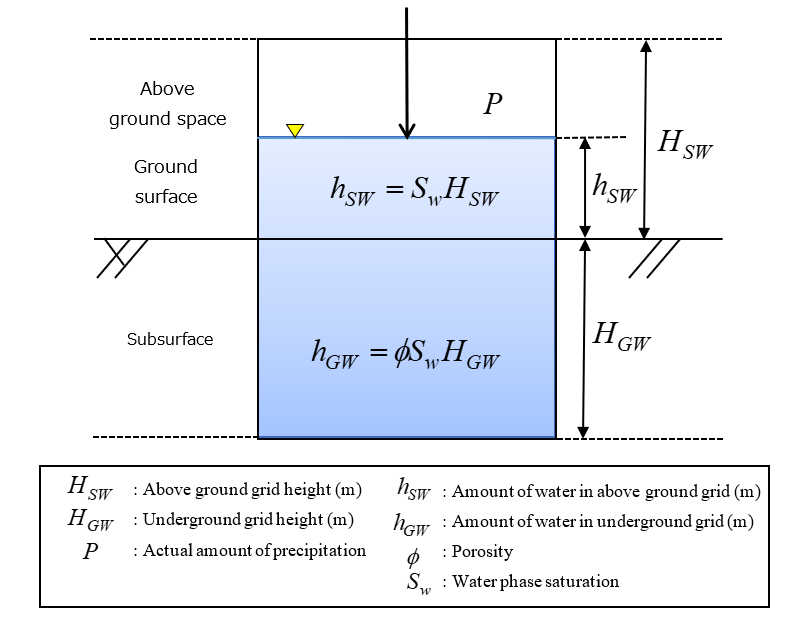
Fig. 2.1 shows a schematic diagram of the water state near the ground surface at some point in time. Surface water exists in the above-ground space, and the subsurface is considered to be saturated with groundwater to some depth, and these are represented by analytical grids of heights \(h_{\text{SW}}\) and \(h_{\text{GW}}\) respectively. The amounts of water in the surface and subsurface grids in this state are represented by the product of the respective grids’ heights, degree of saturation of the water phase, and effective porosity. The above-ground grid is considered to be a free space with an effective porosity of 1.0. If the amount of evapotranspiration input at this time is less than the amount of surface water at the site, evapotranspiration occurs within only the above-ground grid. If there is not enough water in the above-ground grid, evaporation is added from the ground immediately beneath. This soil evaporation corresponds to some degree to the amount of water in the pores, and is evaluated according to the evaporation rate data, which are represented by a nonlinear function of the degree of saturation of the water phase. Furthermore, the amount of water that is missing even after adding this soil evaporation is not considered, and the following amount is treated as the upper limit in the calculation.
\[E_{p} = h_{\text{SW}} + h_{\text{GW}}\begin{matrix} & \left( E_{p} \geq h_{\text{SW}} + h_{\text{GW}} \right) \end{matrix}\qquad{(2.3)}\]
The calculation of the amount of evapotranspiration differs depending on factors such as the above-ground air temperature, land use, sunlight, and coverage status; several models are known for estimating the amount (Hamon 1961) (Penman 1948) (Haith 1987). Because no particular evapotranspiration estimation model is employed in GETFLOWS, evapotranspiration quantities that have been evaluated in advance by the evaluator can be freely input. This also makes it easy to use the calculation results of a tank model that takes into account interception effects that depend on the state of the canopy and forest floor.
Surface Flows
Equations of Motion and Equations of Continuity for Open Channels
Equations of motion
Surface water flows in rivers and on mountain sides are modeled as open-channel flows. Let us now consider the behavior of a body of water flowing in an open-channel of uniform slope, as shown in Figs. 2-3 and 2-4 (the body of water between A and B in the cross section of the water flow). If the water depth is assumed to be sufficiently small compared to the channel width, an averaged shallow water flow approximation can be applied in the vertical direction. The driving forces behind the water flow are the terrain gradient and the water depth gradient, and by adding the contributions from friction acting from the bottom surface and external inputs and outputs, the equations of motion can be expressed as follows.
\[ \beta\frac{1}{g}\frac{\partial v_{x}}{\partial t} = \frac{\partial\xi}{\partial x} - \frac{\partial h}{\partial x}\cos^{2}\theta_{x} - \frac{\partial h_{\text{fx}}}{\partial x} - \frac{\alpha}{2g}\frac{\partial{v_{}}^{2}}{\partial x} - \frac{P_{r}v_{x}}{\text{gh}} \qquad{(2.4)}\]
Here, the symbols have the following meanings.
| \(\theta_{x},\theta_{y}\) | Slope gradient in each flow direction \(\lbrack - \rbrack\) |
| \(h\) | Water depth \(\lbrack L\rbrack\) |
| \(h_{\text{fx}},h_{\text{fy}}\) | Friction losses in each flow direction \(\lbrack - \rbrack\) |
| \(v_{x},v_{y}\) | Flow velocity in each flow direction averaged over water depth \(\lbrack LT^{- 1}\rbrack\) |
| \(\xi\) | Open channel height \(\lbrack L\rbrack\) |
| \(\alpha\) | Energy correction coefficient \(\lbrack - \rbrack\) |
| \(\beta\) | Momentum correction coefficient \(\lbrack - \rbrack\) |
| \(P_{r}\) | Amount of precipitation \(\lbrack LT^{- 1}\rbrack\) |
| \(g\) | Acceleration of gravity \(\lbrack LT^{- 2}\rbrack\) |
| \(t\) | Time \(\lbrack T\rbrack\) |
| \(x,y\) | Distances of the flow direction components \(\lbrack L\rbrack\) |
The first term on the right-hand side of the above equation represents the driving force from the slope gradient, the second term represents the driving force from the water depth gradient, the third term represents the drag force due to friction (friction loss gradient), the fourth term represents the net momentum (velocity term), and the fifth term represents the loss of momentum due to rainfall. The left-hand side represents the change in velocity (inertia term) of the water flow that occurs as a consequence of these external forces.

Equations of continuity
The equation for the conservation of mass of a body of water flowing in a channel where the width is not constant can be expressed as follows for each of the flow direction components.
\[\frac{\partial\rho\text{v}_{x}A_{x}}{\partial x} + \frac{\partial\rho\text{A}_{x}}{\partial t} = 0\qquad{(2.5)}\]
Here, \(\rho\) is the density of water and \(A_{x}\) is the cross-sectional area \(\left( L^{2} \right)\) in the \(x\) direction. In particular, when the flow channel width \(W_{i}\left( \ i = x,y \right)\) is constant, \(A_{x} = Wh\) and the above equation can be expressed as follows.
\[\frac{\partial\left( v_{x}h \right)}{\partial x} + \frac{\partial h}{\partial t} = 0\qquad{(2.6)}\]
Formula for Average Flow Velocity
From experiments on open channels, it is known that the following average flow velocity formula (the Manning formula) is satisfied under conditions of uniform flow where the flow direction component of the weight of the body of water is in equilibrium with the friction drag along the channel walls.
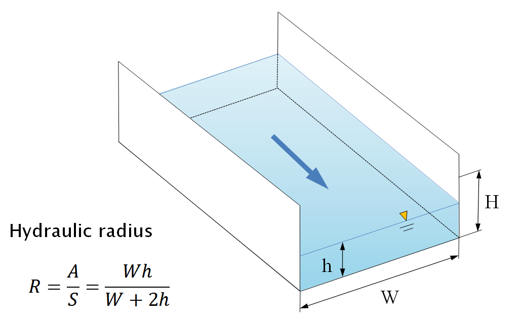
\[v = \frac{R^{2/3}}{n}\sqrt{\frac{\partial\xi}{\partial x}} = \frac{R^{2/3}}{n}\sqrt{i_{g}}\qquad{(2.7)}\]
Here, R is the hydraulic radius, which represents the hydraulic water depth, and is defined by the relation shown in Fig. 2.2 by using the flow channel cross-sectional area A and wetted perimeter \(S\); \(i_{g}\) represents the flow-channel-floor gradient \(\partial\eta/\partial x\) in the flow direction, and \(n\) is Manning’s roughness coefficient, which is assigned separately to the individual calculation cells according to the river bed shape and material, surface vegetation (forest, grass field, dry field, etc.), and artificial coverage (pavement, etc.). Manning’s roughness coefficient has dimensions of \(L^{- 1/3}T\) (or in SI units, s/m3).
Approximation Formulas for Open-channel Flow
In principle, the water depth and velocity can be obtained at any location, and the behavior of the surface water can be tracked by simultaneously solving the equations of motion and continuity shown above. However, although the equations of motion can be solved as-is, the timesteps need to be small, and the equations as written cannot be used for predications on the time scales of actual river problems. An approximation that simplifies the equations of motion by considering only the main contributions is therefore used instead.
Table 2.2 shows the proportions of the magnitudes of each of the terms in the surface water equations of motions shown in Equ. 2.4 as a fraction of 100% of the total for various types of flows. This calculation is as discussed by Sekine (2005) on the basis of the results of actual instantaneous measurements of flows ((Gunaratnum 1970), (Sekine 2005)).
| Type | Inertia term \[\beta\frac{1}{g}\frac{\partial v_{x}}{\partial t}\] | Velocity term \[\frac{\alpha}{2g}\frac{\partial{v_{x}}^{2}}{\partial x}\] | Pressure term \[\frac{\partial h}{\partial x}\cos^{2}\theta_{x}\] | Gravity term \[\frac{\partial\xi}{\partial x}\] | Friction term \[\frac{\partial h_{\text{fx}}}{\partial x}\] |
|---|---|---|---|---|---|
| River | 0.10 | 0.30 | 0.91 | 49.80 | 48.89 |
| Artificial channel | 0.36 | 0.36 | 72.53 | 13.45 | 13.30 |
| Surface water | 0.37 | 0.37 | 3.70 | 47.78 | 47.78 |
From this, it is clear that the sum of the pressure term, gravity term, and friction term accounts for over 99% for all types, and that the contributions of the inertia term and velocity term are less than 1% together. The following two approximations are therefore typically used in practice.
Kinematic wave approximation
The kinematic wave approximation assumes steady state flow of the body of water over small time intervals and considers the uniform flow state, in which the slope gradient and friction gradient in the equations of motion are in equilibrium:
\[\frac{\partial\xi}{\partial x} - \frac{\partial h_{f}}{\partial x} = 0\qquad{(2.8)}\]
When the Manning formula for uniform-flow average flow velocity, as described above, is used, the resulting approximation can be expressed as follows.
\[\frac{v^{2}n^{2}}{R^{4/3}} - \frac{\partial\varepsilon}{\partial x} = 0\qquad{(2.9)}\]
Generalizing this as a flow rate formula that takes the flow direction components into account gives the following equation:
\[Q_{w,x} = v_{x}W_{x}h = - \frac{W_{x}h}{n}{R_{x}}^{\frac{2}{3}}\sqrt{\left| \frac{\partial\xi}{\partial x} \right|}\text{sgn}\left( \frac{\partial\xi}{\partial x} \right)\qquad{(2.10)}\]
Here, \(\text{sgn}( )\) represents the positive or negative sign, determined from the friction loss gradient, and takes a value of 1 when the friction loss gradient is positive and –1 when it is negative.
Although this approximation is suitable for calculating single-slope channel flows for practical use, it does not include terms for flood wave attenuation and deformation. As a result, on slopes with piecewise changes in gradient, inappropriate solutions appear at the points of slope change (Tosaka 2006). Furthermore, this approximation is not suitable for representing locations where the slope gradient is gentle, the wave propagation velocity is small and the water depth gradient cannot be ignored.
Diffusion wave approximation
The diffusion wave approximation is based on the following equation of motion, which also takes the water depth gradient into account.
\[\frac{\partial h}{\partial x}\cos^{2}\theta - \frac{v^{2}n^{2}}{R^{4/3}} - \frac{\partial h_{f}}{\partial x} = 0\qquad{(2.11)}\]
Using the Manning average flow velocity formula to generalize this as a flow rate formula that takes the flow direction components into account gives the following equation.
\[Q_{w,x} = v_{x}W_{x}h\qquad{(2.12)}\]
\[= \frac{{R_{x}}^{\frac{2}{3}}W_{x}h}{n}\sqrt{\left| \frac{\partial h_{f}}{\partial x} - \frac{\partial h}{\partial x}\cos^{2}\theta \right|}\text{sgn}\left( \frac{\partial h_{f}}{\partial x} - \frac{\partial h}{\partial x}\cos^{2}\theta \right)\]
Because the water depth gradient also acts as a driving force in the diffusion wave approximation, it is suitable for representing flows in locations where the slope has piecewise changes and where the water depth gradient cannot be ignored.
Representation of flood flow by diffusion wave approximation
The two-dimensional surface water flow is expressed as follows by applying the diffusion wave approximation.
\[\beta\frac{1}{g}\frac{\partial v_{x}}{\partial t} = \frac{\partial\xi}{\partial x} - \frac{\partial h}{\partial x}\cos^{2}\theta_{x} - \frac{\partial h_{\text{fx}}}{\partial x} - \frac{\alpha}{2g}\frac{\partial{v_{x}}^{2}}{\partial x} - \frac{P_{r}v_{x}}{\text{gh}}\qquad{(2.13)}\]
Subsurface Fluid Flows
From Saturated Flow to Multi-phase Flow (Generalized Darcy’s Law)
In underground hydrology, the saturated flow of water in a basic porous medium is expressed by Darcy’s law as the following equation.
\[v = \left( \mathbf{-}\mathbf{k}\frac{\partial H}{\partial z} \right)\qquad{(2.14)}\]
Here, \(\mathbf{\text{k\ }}\lbrack m/s\rbrack\) is the permeability coefficient of water and \(H\ \lbrack m\rbrack\) is the total head (the sum of the elevation head Z and the pressure head h). The water flow in the more generalized unsaturated state takes the following form.
\[v = \left( \mathbf{- k}k_{\text{rw}}\frac{\partial H_{w}}{\partial z} \right)\qquad{(2.15)}\]
Here, \(k_{\text{rw}}\ \lbrack - \rbrack\) is the relative permeability coefficient of water, \(H_{w}\ \lbrack m\rbrack\) is the total head of the water, and the pressure head is treated as a function of the volume water content.
In contrast, the generalization of Darcy’s law for applicability to fluids other than water has the following form.
\[v = \left( \mathbf{-}\frac{K}{\mathbf{\mu}}\frac{\partial\Psi_{w}}{\partial z} \right)\qquad{(2.16)}\]
In this equation, \(K\ \lbrack m^{2}\rbrack\) is the permeability, \(\mu\ \lbrack\text{Pa} s\rbrack\) is the coefficient of viscosity, and \(\Psi\ \lbrack\text{Pa}\rbrack\) is the hydraulic potential, which can be expressed in terms of pressure and position as follows.
\[\Psi = P + \rho gZ\qquad{(2.17)}\]
Here, \(\rho\ \lbrack\text{kg}/m^{3}\rbrack\) is the fluid density and \(z\ \lbrack m\rbrack\) is the elevation. In the case of a two-phase flow, the following forms are used for water and air, respectively.
\[v_{w} = \left( \mathbf{-}\frac{Kk_{\text{rw}}}{\mu_{w}}\frac{\partial\Psi_{w}}{\partial z} \right)\qquad{(2.18)}\] \[v_{g} = \left( \mathbf{-}\frac{Kk_{\text{rg}}}{\mu_{g}}\frac{\partial\Psi_{g}}{\partial z} \right)\qquad{(2.19)}\]
GETFLOWS is able to handle a generalized treatment of up to three-phase systems by using the flow equations of a generalized two-phase air and water system.
Governing Equations for Two-phase Flow
The governing equations for two-phase air and water flows can be expressed as follows.
\[\nabla \bullet \left( \rho_{w}\frac{Kk_{\text{rw}}}{\mu_{w}}\nabla\Psi_{w} \right) - \rho_{\text{wS}}q_{\text{wS}} = \frac{\partial}{\partial t}\left( \rho_{w}\phi S_{w} \right)\qquad{(2.20)}\]
\[\nabla \bullet \left( \rho_{g}\frac{Kk_{\text{rg}}}{\mu_{g}}\nabla\Psi_{g} \right) - {\rho_{\text{gS}}q}_{\text{gS}} = \frac{\partial}{\partial t}\left( \rho_{g}\phi S_{g} \right)\qquad{(2.21)}\]
The above equations represent the law of conservation of mass for water and air in porous media. The first term on the left-hand side of each equation is the flow term (advection term), the second term is the production term, and the right-hand side is the storage term. The symbols in the equations have the following meanings.
| \(K\) | Absolute permeability \(\lbrack m^{2}\rbrack\) |
| \(\mu_{p}\) | Coefficient of viscosity of the fluid \(p( = w,g,n)\) \(\lbrack Pa s\rbrack\) |
| \(\rho_{p}\) | Density of the fluid phase \(p( = w,g,n)\) \(\lbrack\text{kg}/m^{3}\)] |
| \(\Psi_{p}\) | Potential of the fluid phase \(p\left( = w,g,n \right)\) \(\lbrack\text{Pa}\rbrack\) |
| \(\phi\) | Porosity \(\lbrack - \rbrack\) |
| \(t\) | Time \(\lbrack s\rbrack\) |
| \(q_{\text{pS}}\) | Production and extinction of the fluid phase \(p\left( = w,g,n \right)\) \(\lbrack m^{3}/(m^{3} s)\rbrack\) |
Note that the permeability and relative permeability in the above equations are directional and are tensor quantities (3 × 3 matrices). The potentials of the water phase and air phase in the above equations are expressed by the following equations.
\[\Psi_{w} = P_{g}{- P_{\text{cw}} + \rho}_{w}\text{gZ}\qquad{(2.22)}\] \[\Psi_{g} = P_{g}{+ \rho}_{g}\text{gZ}\qquad{(2.23)}\]
Here, \(P_{g}\) is the air phase pressure, \(P_{\text{cw}}\) is the capillary pressure, and \(Z\) is the elevation (distance, taking up as the positive direction). Furthermore, the following relation exists between the saturations.
\[S_{w} + S_{g} = 1\qquad{(2.24)}\]
The unknown variables in the above equations are the air phase pressure \(P_{g}\) and the water saturation \(S_{w}\), and the simulator solves for these by a simultaneous fully implicit method.
Differences between Saturated–Unsaturated Groundwater Analysis and Two-phase Analysis
In typical groundwater analyses, groundwater flows in shallow underground areas are formulated as “flows of water in the unsaturated state,” and air that exists and moves at the same time is not considered. This method is called saturated–unsaturated analysis and uses the following governing equation.
\[\nabla \bullet \left( \mathbf{k}k_{\text{rw}}\nabla(h + z) \right) - q_{\text{wS}} = \left( {C + S}_{w}S_{s} \right)\frac{\partial h}{\partial t}\qquad{(2.25)}\]
Here, \(k\) is the permeability coefficient of water, \(h\) is the pressure head, \(z\) is the elevation, \(C\) is the specific water capacity, and \(S_{s}\) is the specific storage coefficient, with the latter two defined as follows.
\[C = \frac{\partial\phi S_{w}}{\partial h},\ S_{S} = \phi(c_{w} + c_{\phi})\qquad{(2.26)}\]
Although this equation is equivalent to the law of conservation of mass of water in two-phase flow, the right-hand side expands to give the head. The formulation as saturated–-unsaturated flow and the formulation as two-phase flow in the equations are thought to obtain nearly identical results in the unsaturated range, where the air pressure is close to atmospheric pressure. Because two-phase flow also models the gas phase at the same time, it can be used for conditions where high pressures exist (for example, geological conditions in which the gas has become blocked or gas has been injected at high pressure) and to calculate phenomena such as dissolution and volatilization. Refer to (Tosaka 2006) for details.
Fully Coupled Surface and Subsurface Flows
In continental-scale hydrological cycles, surface flow and underground permeation, which are obtained from the precipitation input to the surface, are in constant interchange via permeation from the surface to underground and upwelling of water from underground to the surface. River water being supported by discharges of groundwater during periods of no rainfall is a good example of this.
However, since the difference in velocity is extremely large between surface flows and subsurface flows and the forms of the equations differ between the two, river research and groundwater research have conventionally been performed as different fields. Because of this, in cases where interactions between the two are considered, some artificial assumptions need to be made to estimate the source terms.
GETFLOWS employs a procedure that solves the flows in a fully unified way by using a generalized flow formula that gives a common numerical description of the surface and subsurface without decoupling them. This section gives a basic description of the procedure.
Generalized Flow Equation for Surface and Subsurface Flows
The average flow velocity formula for surface flows and the multi-phase Darcy’s law for subsurface fluids can both be generalized to the following nonlinear flow formula.
\[Q = {- K}^{*} \bullet A^{*} \bullet f_{1}\left\lbrack P_{w} \right\rbrack{\bullet f}_{2}\left\lbrack S_{w} \right\rbrack \bullet f_{3}\left\lbrack P_{w},S_{w} \right\rbrack\qquad{(2.27)}\]
Although this relation is basically equivalent to the subsurface multi-phase flow equation, it also incorporates the subsurface flow equation. Functions \(f_{1},\ f_{2},\) and \(f_{3}\) are nonlinear functions of water pressure and degree of saturation, and are given by the specific forms shown in Table 2.3. If we now consider a one-dimensional open-channel water flow in a channel of constant width \(W\) and constant height \(H\), then each of the components of the above equation, Darcy’s law for groundwater, and the diffusion wave approximation for surface water are calculated as the functions shown in Table 2.3, (Tosaka 2000). The product of the components, arranged vertically in the table, represents the average flow rate along the flow.
| Darcy’s law | Diffusion wave approximation | Linearized diffusion wave approximation | |
|---|---|---|---|
| \(K^{*}\) | \(K_{x}\) | \(\frac{\mu_{w}}{\rho_{w}\text{gn}}\left( \frac{\text{WH}}{2H + W} \right)^{\frac{2}{3}}\) | \(\frac{\mu_{w}}{\rho_{w}\text{gn}\sqrt{\left| i_{g} \right|}}\left( \frac{\text{WH}}{2H + W} \right)^{\frac{2}{3}}\) |
| \(A^{*}\) | \(\text{WH}\) | \(\text{WH}\) | \(\text{WH}\) |
| \(f_{1}\left\lbrack P_{w} \right\rbrack\) | \(\frac{\rho_{w}}{\mu_{w}}\) | \(\frac{\rho_{w}}{\mu_{w}}\) | \(\frac{\rho_{w}}{\mu_{w}}\) |
| \(f_{2}\left\lbrack S_{w} \right\rbrack\) | \(k_{\text{rw}}\) | \({S_{w}}^{\frac{5}{3}}\left( \frac{2H + W}{2S_{w}H + W} \right)^{\frac{2}{3}}\) | \({S_{w}}^{\frac{5}{3}}\left( \frac{2H + W}{2S_{w}H + W} \right)^{\frac{2}{3}}\) |
| \(f_{3}\left\lbrack P_{w},S_{w} \right\rbrack\) | \(\frac{\partial\Psi_{w}}{\partial x}\) | \(\left( \rho_{w}g \right)^{\frac{1}{2}}\sqrt{\left| \frac{\partial\Psi_{w}}{\partial x} \right|}\text{sgn}\left( \frac{\partial\Psi_{w}}{\partial x} \right)\) | \(\frac{\partial\Psi_{w}}{\partial x}\) |
In the surface flow calculation, the diffusion wave approximation may be numerically unstable as written. In GETFLOWS, a linearized diffusion wave approximation can be used, which approximates more parts of the diffusion wave equation (Tosaka 2000).
The width \(W\) and height \(H\) of the flow correspond to the width and height of the grid when the space is discretized, and the water depth \(h\) in the grid is given by \(h = S_{w}H\) from the degree of saturation of the water phase.
The above relation can be applied in the same way for other purposes, which allows uniform treatment of the water phase, air phase, NAPL, dissolved substances in river water, and heat transport.
Interchange between Surface Water and Groundwater
In GETFLOWS, interchange phenomena between surface and subsurface fluids such as water and air (for example, permeation by a body of water or by rainfall and the infiltration or exfiltration of air that accompanies it) are modeled as follows.
Let us now consider the state near the surface. This state comprises the atmosphere, surface water, and surface soil, as shown in Fig. 2.4, and is represented by neighboring grids of heights H1 and H2 with the land surface as the boundary. The surface grid (site 1) contains the atmosphere and surface water and has a pressure \(P_{g1}\) and surface water depth \(h\). In the subsurface grid (site 2), the pores within the ground layer are saturated with water. The permeability of each site is represented by K1 and K2 for the surface and subsurface grids, respectively, with the permeability of the above-ground grid considered to be extremely large (i.e., \(K_{1} \gg K_{2}\)). The amount of flow passing between the two sites is calculated from the following formula.
\[Q_{z} = - \frac{K_{12}k_{rw12}}{\mu_{w}}A_{12}\frac{\partial\Psi_{w}}{\partial z}\qquad{(2.28)}\]
Here, \(K_{12}\) is the average permeability between both grids, \(k_{rw12}\) is the relative permeability of water, and \(A_{12}\) is the area of the grids together. Furthermore, the potential difference between the two points is calculated using the following equation and taking the upward direction as positive (\(+ z\)).
\[{\Delta\Psi}_{w} = \Psi_{w1} - \Psi_{w2} = \left( P_{w1} + \rho_{w}\text{gd}z_{1} \right) - \left( P_{w2} + \rho_{w}g\left( - dz_{2} \right) \right) = P_{w1} + \rho_{w}g\left( dz_{1} + dz_{2} \right) - P_{w2}\qquad{(2.29)}\]
Here, \(dz_{1} = H_{1}/2\) and \(dz_{2} = H_{2}/2\). Using this relation, the amount of flow between the grids can be expressed as follows.
\[Q_{z} = - \frac{K_{12}k_{rw12}}{\mu_{w}}A_{12}\frac{P_{w1} + \rho_{w}g\left( dz_{1} + dz_{2} \right) - P_{w2}}{dz_{1} + dz_{2}}\qquad{(2.30)}\]
The average permeability between the grids is expressed by the following equation for the harmonic mean of the permeabilities of each of the grids.
\[K_{12} = - \frac{dz_{1} + dz_{2}}{\frac{dz_{1}}{K_{1}} + \frac{dz_{2}}{K_{2}}}\qquad{(2.31)}\]
Writing the water pressure in the surface grid (site 1) in the same form as the subsurface pressure gives \({P_{w1} = P_{g1} - P}_{c}^{*}\). Because the specific form of the potential difference between the two sites can be expressed by \(P_{g1} + \rho_{w}gh + \rho_{w}\text{gd}z_{2} - P_{w2}\), the following relation must be satisfied for the relation with the * equation.
\[P_{g1} + \rho_{w}gh + \rho_{w}\text{gd}z_{2} - P_{w2} = {P_{g1} - P}_{c}^{*} + \rho_{w}g\left( dz_{1} + dz_{2} \right) - P_{w2}\qquad{(2.32)}\]
This gives the following relation for \(P_{c}^{*}\).
\[P_{c}^{*} = - \rho_{w}\text{gH}\left( 0.5 - S_{w} \right)\qquad{(2.33)}\]
This differs from the hydraulic capillary pressure in the subsurface layer, and is thus called the pseudo-capillary pressure (Tosaka 1996). Fig. 2.5 shows the shape of the pseudo-capillary pressure curve.
The relative permeability \(k_{rw12}\) between two sites differs depending on whether there is permeation or discharge. When the flow is from the surface (permeation), the capacity of the above-ground space is extremely large, and so the air phase does not interfere with the behavior of the water (e.g., upwelling or permeation), and we always have \(k_{rw12} = 1\). In the case of discharge, the relative permeability of the first subsurface layer is used.


Extended Numerical Representation of the Water Circulation System
This chapter looks at extensions to the basic representations from Chapter 2. These can be used to represent a wider variety of phenomena.
Extension of Isothermal Flow
Two-Phase Flow with Consideration of Dissolved Air
GETFLOWS is able to analyze the dissolution of the air phase into the water phase and the transport and diffusion behavior of the dissolved air as a two-phase water and air system. This analytical capability is often used when investigating aerobic and anaerobic atmospheres in ground layers resulting from the distribution of dissolved air in shallow groundwater near the ground surface and when analyzing the behavior of compressed gas in storage layers deep underground.
If we add an interphase mass transfer term, representing the dissolution and release of air into and out of the water phase, to a two-phase water and air flow equation in a porous medium in an isothermal state, the governing equations of the two-phase three-component (water, air, dissolved air) fluid system can be described by the following equations.
\[\nabla \bullet \left( \rho_{\text{wS}}\frac{Kk_{\text{rw}}}{\mu_{w}B_{w}}\nabla\Psi_{w} \right) - \rho_{\text{wS}}q_{\text{wS}} = \frac{\partial}{\partial t}\left( \rho_{\text{wS}}\phi\frac{S_{w}}{B_{w}} \right)\qquad{(3.1)}\] \[\nabla \bullet \left( \rho_{\text{gS}}\frac{Kk_{\text{rg}}}{\mu_{g}B_{g}}\nabla\Psi_{g} \right) + m_{g \rightarrow w} - {\rho_{\text{gS}}q}_{\text{gS}} = \frac{\partial}{\partial t}\left( \rho_{\text{gS}}\phi\frac{S_{g}}{B_{g}} \right)\qquad{(3.2)}\] \[\nabla \bullet \left( \rho_{\text{wS}}\frac{Kk_{\text{rw}}R_{\text{da}}}{\mu_{w}B_{w}}\nabla\Psi_{w} \right) + \nabla{\bullet D}_{\text{da}}\nabla\left( \rho_{\text{wS}}\frac{R_{\text{da}}}{B_{w}} \right) - m_{g \rightarrow w} - \rho_{\text{wS}}q_{\text{wS}}R_{\text{da}} = \frac{\partial}{\partial t}\left( \rho_{\text{wS}}\phi\frac{S_{w}R_{\text{da}}}{B_{w}} \right)\qquad{(3.3)}\]
The symbols have the following meanings.
| \(K\) | Absolute permeability \(\lbrack m^{2}\rbrack\) |
| \(S_{p}\) | Degree of saturation of the fluid phase \(p = w,g\) \(\lbrack - \rbrack\) |
| \(\mu_{p}\) | Coefficient of viscosity of the fluid phase \(p = w,g\) \(\lbrack Pa s\rbrack\) |
| \(\rho_{p}\) | Density of the fluid phase \(p( = w,g)\) \(\lbrack kg/m^{3}\rbrack\) |
| \(B_{p}\) | Capacity coefficient of the fluid phase \(p( = w,g)\) \(\lbrack m^{3}/m^{3}\rbrack\) |
| \(\Psi_{p}\) | Potential of the fluid phase \(p = w,g\) \(\lbrack Pa\rbrack\) |
| \(\phi\) | Porosity \(\lbrack - \rbrack\) |
| \(R_{\text{da}}\) | Concentration of the air component dissolved in the water phase \(\lbrack m^{3}/m^{3}\rbrack\) |
| \(D_{\text{da}}\) | Hydrodynamic dispersion coefficient of dissolved air \(\lbrack m^{2} s^{- 1}\rbrack\) |
| \(m_{g \rightarrow w}\) | Dissolution and liberation term for the air phase in the water phase \(\lbrack kg/{(m}^{3} s^{})\rbrack\) |
The solubility of air in water is pressure-dependent, and the viscosity and compressibility of water that contains dissolved air are also pressure-dependent. The degree of nonlinearity of the dependence of the fluid physical properties on pressure varies discontinuously at the boundary formed by the bubble point pressure. GETFLOWS performs two-phase fluid analysis that takes into account variations in the physical properties of the fluids and variations in lability in the porous medium. The specific treatment of the successive updating of the physical properties of the fluids is described later.
An additional choice is available for the dissolution of air into the water phase (interphase transfer phenomenon) between equilibrium theory (which tracks the pressure state as it changes from moment to moment and reaches the saturation concentration instantaneously) and kinetic theory (which takes into account the unsteady movement between equilibrium states).
Handling of dissolved gas + solubility and viscosity coefficient
Three-phase Flow Including a Solute or NAPL
By further generalizing the system of fluids, the following phases can be consider: a gas phase, a liquid water phase, and an NAPL phase, which is a water-insoluble liquid phase. Furthermore, governing equations can be established that include the dissolution into water and volatilization into the gas phase that occur from the NAPL.
In GETFLOWS, the basic equations are three-phase flow equations generalized to the following forms.
\[\nabla \bullet \left( \rho_{w}\frac{Kk_{\text{rw}}}{\mu_{w}}\nabla\Psi_{w} \right) - \rho_{\text{wS}}q_{\text{wS}} = \frac{\partial}{\partial t}\left( \rho_{w}\phi S_{w} \right)\qquad{(3.4)}\] \[\nabla \bullet \left( \rho_{g}\frac{Kk_{\text{rg}}}{\mu_{g}}\nabla\Psi_{g} \right) - {\rho_{\text{gS}}q}_{\text{gS}} = \frac{\partial}{\partial t}\left( \rho_{g}\phi S_{g} \right)\qquad{(3.5)}\] \[\nabla \bullet \left( \rho_{\text{nS}}\frac{Kk_{\text{rn}}}{\mu_{n}B_{n}}\nabla\Psi_{n} \right) - {\rho_{\text{nS}}q}_{\text{nS}} - m_{n \rightarrow w} - m_{n \rightarrow g} = \frac{\partial}{\partial t}\left( \rho_{\text{nS}}\phi\frac{S_{n}}{B_{n}} \right)\qquad{(3.6)}\] \[\nabla \bullet \left( \rho_{\text{wS}}\frac{Kk_{\text{rw}}R_{w}}{\mu_{w}B_{w}}\nabla\Psi_{w} \right) + \nabla{\bullet D}_{w}\nabla\left( \rho_{\text{wS}}\frac{R_{w}}{B_{w}} \right) - \rho_{\text{wS}}q_{\text{wS}}R_{w} + m_{n \rightarrow w} - m_{w \rightarrow s} = \frac{\partial}{\partial t}\left( \rho_{\text{wS}}\phi\frac{S_{w}R_{w}}{B_{w}} \right)\qquad{(3.7)}\] \[\nabla \bullet \left( \rho_{\text{gS}}\frac{Kk_{\text{rg}}R_{g}}{\mu_{g}B_{g}}\nabla\Psi_{g} \right) + \nabla{\bullet D}_{g}\nabla\left( \rho_{\text{gS}}\frac{R_{g}}{B_{g}} \right) - {\rho_{\text{gS}}q}_{\text{gS}}R_{g} + m_{n \rightarrow g} - m_{g \rightarrow s} = \frac{\partial}{\partial t}\left( \rho_{\text{gS}}\phi\frac{S_{g}R_{g}}{B_{g}} \right)\qquad{(3.8)}\]
In these expressions, the symbols have the following meanings.
| \(\rho_{pS}\) \(B_{p}\) | Density of the fluid phase \(p( = w,g,n)\) at standard temperature and pressure \(\lbrack\text{kg}/m^{3}\rbrack\) Capacity coefficient of the fluid phase \(p\left( = w,g,n \right)\) \(\lbrack - \rbrack\) |
| \(D_{p}\) | Hydrodynamic dispersion coefficient of the fluid phase \(p\left( = w,g \right)\) \(\lbrack m^{2}/s\rbrack\) |
| \(R_{w}\) | Volume concentration of dissolved matter in the water phase \(\lbrack - \rbrack\) |
| \(R_{g}\) | Volume concentration of volatilized matter in the air phase \(\lbrack - \rbrack\) |
| \(m_{n \rightarrow w}\) | Amount of dissolution of the NAPL phase into the water phase \(\lbrack kg/(m^{3} s^{})\rbrack\) |
| \(m_{n \rightarrow g}\) | Amount of volatilization of the NAPL phase into the air phase \(\lbrack kg/(m^{3} s)\rbrack\) |
| \(m_{p \rightarrow s}\) | Amount of adsorption of the fluid phase \(p\left( = w,g \right)\) onto the solid phase \(\lbrack kg/(m^{3} s)\rbrack\) |
That is, the total volume of the fluid in the void is constrained by the following relationship regarding the degree of saturation.
\[\Psi_{w} = P_{w}{+ \rho}_{w}\text{gZ}\qquad{(3.9)}\] \[\Psi_{g} = P_{g}{+ \rho}_{g}\text{gZ}\qquad{(3.10)}\] \[\Psi_{n} = P_{n}{+ \rho}_{n}\text{gZ}\qquad{(3.11)}\]
Furthermore, the capillary pressures that act between the water and NAPL phases and between the air and NAPL phases in the three-phase system can be expressed as follows.
\[P_{c,w} = P_{n} - P_{w}\left( S_{w} \right)\qquad{(3.12)}\] \[P_{c,g} = P_{g}\left( S_{g} \right) - P_{n}\qquad{(3.13)}\]
Here, \(P_{c,w}\) is the capillary pressure between the water and NAPL phases and \(P_{c,g}\) is the capillary pressure between the air and NAPL phases. Notation such as \(P_{w}\left( S_{w} \right)\) in the equations indicates that the water phase pressure \(P_{w}\) is a function of the degree of saturation \(S_{w}\). The initially unknown variables that are ultimately found are \(P_{n}\), \(S_{w}\), \(S_{g}\), \(R_{w}\), and \(R_{g}\). The governing equations for flows in non-isothermal states are described later.
The third term on the left side of the equations {Equ. 2.20} {Equ. 2.21} is the production phase of the water phase, the air phase, NAPL, the second term on the left side of the equation.
The term is the diffusion term of the substance, and the third term is the term of substance creation / disappearance caused by the production and pressing of the fluid phase. Intermolecular mass transfer due to dissolution and volatilization of NAPL is represented by the symbol \(m\) in the equation.
The explanation of the symbols in the formula is as follows.
The unknown variables in the above equation are the pressure of each fluid phase \(P_{w}, P_{g}, P_{n}\), saturation \(S_{w}, S_{g}, S_{n}\), the substance concentration in the aqueous phase \(R_{w}\), and the substance concentration in the air phase (\(R_{g}\). It is not solvable as it is.
In GETFLOWS, unknown variables are reduced to five by using the relational expression of the fluid saturation in the air gap and the following relation relating to the capillary pressure. These reductions are made simultaneous to obtain a numerical solution.
Treatment of hydrodynamic dispersion
In solute transport in porous media, the hydrodynamic dispersion that occurs due to the non-uniformity of the pore flow channel needs to be taken into account. GETFLOWS employs a method that determines the solute concentration by solving the advection-dispersion equation (by the upwind method) simultaneously with calculating the water and air flows.
The following general forms, which are proportional to the velocities and concentration gradients of the flows in the soil and solid rock, are used for the coefficient of dispersion for the mass component \(i\) of the solute transport fluid phase \(p\).
\[D_{p,x,i} = \text{De}_{p,i} + \alpha_{L}\frac{{v_{p,x}}^{2}}{V_{p}} + \alpha_{T}\frac{{v_{p,y}}^{2}}{V_{p}} + \alpha_{T}\frac{{v_{p,z}}^{2}}{V_{p}}\qquad{(3.14)}\] \[D_{p,y,i} = \text{De}_{p,i} + \alpha_{T}\frac{{v_{p,x}}^{2}}{V_{p}} + \alpha_{L}\frac{{v_{p,y}}^{2}}{V_{p}} + \alpha_{T}\frac{{v_{p,z}}^{2}}{V_{p}}\qquad{(3.15)}\] \[D_{p,z,i} = \text{De}_{p,i} + \alpha_{T}\frac{{v_{p,x}}^{2}}{V_{p}} + \alpha_{T}\frac{{v_{p,y}}^{2}}{V_{p}} + \alpha_{L}\frac{{v_{p,z}}^{2}}{V_{p}}\qquad{(3.16)}\] \[V_{p} = \sqrt{{v_{p,x}}^{2} + {v_{p,y}}^{2} + {v_{p,z}}^{2}}\qquad{(3.17)}\]
Here, \(\alpha_{L}\) and \(\alpha_{T}\) are the vertical dispersion length [L] and horizontal dispersion length [L], \(\text{De}_{p,i}\) is the effective diffusion coefficient [L2T-1] for the mass component \(i\) of fluid phase \(p\) with the pore structure of the porous medium taken into account for the molecular diffusion coefficient in free water for each mass component; \(v_{p,x}\), \(v_{p,y}\), and \(v_{p,z}\) are the directional components of the Darcy [LT-1] of the fluid phase. Although the off-diagonal components (\(D_{p,xy,i}\), \(D_{p,yz,i}\), etc.) of the dispersion coefficient tensor are included in the calculation mathematically, they are basically ignored at the current point in time.
About the improvements to solute transport
The upwind method is widely used because it is extremely stable, conservative, and produces smooth solutions without artifacts. However, under conditions where the discretization is coarse and the velocity is large, the dispersion that is calculated (numerical dispersion) is larger than the dispersion of the medium, which makes the solution unreliable.
It is thought that the advection-dispersion problem, in which variations in density do not occur at low solute concentrations, can be solved by first calculating the flow field and obtaining the velocity vector at each point and then solving the advection-dispersion equations by a method that has low numerical dispersion. Examples of previous methods that have been studied include the method of characteristics, the mark and cell method, the total variation diminishing scheme with cubic interpolation, and multi-dimensional conservative cubic interpolated profile methods. These are discussed separately.
Heat and Water Circulation Model (Matter and Energy Transport Model)
In general continental water cycle modeling, isothermal conditions are assumed and analysis is performed by ignoring temperature variations. However, evapotranspiration varies greatly with seasonal surface temperature variations, and it is often necessary to take into account the additional effect of geothermal heat in the analysis of deep subsurface areas. To explain the observed values of the changes in river water temperatures and changes in groundwater temperatures, an analysis procedure that takes heat flows into account is necessary.
GETFLOWS is able to treat heat transport with these kinds of materials. The governing equations of flows under non-isothermal conditions consist of fluid phase and solid phase energy conservation equations in addition to water phase and air phase mass balance equations. When the phenomena of phase changes in the water phase (generation of water vapor and condensation), water vapor transportation in the air phase, and heat exchange between the fluid phases and solid phase occurring due to due to variations in temperature are taken into account, the following governing equations for two-phase water and air flows under non-isothermal conditions are obtained.
\[\nabla \bullet \left( \rho_{w}v\frac{Kk_{\text{rw}}}{\mu_{w}B_{w}}\nabla\Psi_{w} \right) - m_{w \rightarrow g} - \rho_{wS}q_{\text{wS}} = \frac{\partial}{\partial t}\left( \rho_{\text{wS}}\phi\frac{S_{w}}{B_{w}} \right)\qquad{(3.18)}\]
\[\nabla \bullet \left( \rho_{\text{gS}}\frac{Kk_{\text{rg}}}{\mu_{g}B_{g}}\nabla\Psi_{g} \right) - {\rho_{\text{gS}}q}_{\text{gS}} = \frac{\partial}{\partial t}\left( \rho_{\text{gS}}\phi\frac{S_{g}}{B_{g}} \right)\qquad{(3.19)}\]
\[\nabla \bullet \left( \rho_{\text{gS}}\frac{Kk_{\text{rg}}R_{\text{wv}}}{\mu_{g}B_{g}}\nabla\Psi_{g} \right) + \nabla{\bullet D}_{\text{wv}}\nabla\left( \rho_{\text{gS}}\frac{R_{\text{wv}}}{B_{g}} \right) + m_{w \rightarrow g} - {\rho_{\text{gS}}q}_{\text{gS}}R_{\text{wv}} = \frac{\partial}{\partial t}\left( \rho_{\text{gS}}\phi\frac{S_{g}R_{\text{wv}}}{B_{g}} \right)\qquad{(3.20)}\]
\[\nabla \bullet \left( \rho_{\text{wS}}\frac{Kk_{\text{rw}}H_{w}}{\mu_{w}B_{w}}\nabla\Psi_{w} \right) + \nabla \bullet \left( \rho_{\text{gS}}\frac{Kk_{\text{rg}}H_{g}}{\mu_{g}B_{g}}\nabla\Psi_{g} \right) + \nabla \bullet \lambda_{f}\left( \nabla T_{f} \right) + E_{f \longleftrightarrow s} - q_{\text{wS}}H_{w} - q_{\text{gS}}H_{g} = \frac{\partial}{\partial t}\left( \rho_{\text{wS}}\phi\frac{S_{w}U_{w}}{B_{w}} + \rho_{\text{gS}}\phi\frac{S_{g}U_{g}}{B_{g}} \right)\qquad{(3.21)}\]
\[\nabla \bullet \lambda_{s}\left( {\nabla T}_{s} \right)\mathbf{-}E_{f \longleftrightarrow s} - E_{0} = \frac{\partial}{\partial t}\left\lbrack \rho_{s}\left( 1 - \phi \right)U_{s} \right\rbrack\qquad{(3.22)}\]
The above equations represent the mass conservation equations for the water phase, air phase, and water vapor phase, and the energy conservation equations for the fluid phases and solid phase. Heat transport by surface fluids and interactions with subsurface fluids are taken into account in a uniform way by using the generalized flow formula that was described previously.
The symbols used in the equations have the following meanings.
| \(K\) | Absolute permeability \(\lbrack m^{2}\rbrack\) |
| \(S_{p}\) | Degree of saturation of the fluid phase \(p( = w,g)\) \(\lbrack - \rbrack\) |
| \(\mu_{p}\) | Coefficient of viscosity of the fluid phase \(p( = w,g)\) \(\lbrack Pa s\rbrack\) |
| \(\rho_{p}\) | Density of the fluid phase \(p( = w,g,s)\) \(\lbrack kg/m^{3}\rbrack\) |
| \(B_{p}\) | Capacity coefficient of the fluid phase \(p( = w,g)\) \(\lbrack m^{3}/m^{3}\rbrack\) |
| \(\Psi_{p}\) | Potential of the fluid phase \(p\left( = w,g \right)\) \(\lbrack Pa\rbrack\) |
| \(\phi\) | Porosity \(\lbrack - \rbrack\) |
| \(R_{\text{wv}}\) | Water vapor concentration in the air phase \(\lbrack m^{3}/m^{3}\rbrack\) |
| \(D_{\text{wv}}\) | Hydrodynamic dispersion coefficient of the water vapor \(\lbrack m^{2} s^{- 1}\rbrack\) |
| \(H_{p}\) | Entropy of the fluid phase \(p\left( = w,g,n \right)\) \(\lbrack J/kg\rbrack\) |
| \(U_{p}\) | Internal energy of the fluid phase \(p\left( = w,g,n \right)\) \(\lbrack J/kg\rbrack\) |
| \(T_{f}\) | Mean temperature of the fluid phases \(\lbrack C\rbrack\) |
| \(T_{s}\) | Solid phase temperature \(\lbrack C\rbrack\) |
| \(\lambda_{f}\) | Mean thermal conductivity of the fluid phases \(\lbrack J/(K m s)(\rbrack\) |
| \(\lambda_{s}\) | Thermal conductivity of the solid phase \(\lbrack J/(K m s^{})\rbrack\) |
| \(q_{\text{pS}}\) | Rate of production and extinction of the fluid phase \(p\left( = w,g,n \right)\) \(\lbrack kg/(m^{3} s)\rbrack\) |
| \(m_{w \rightarrow g}\) | Water vapor generation and condensation term \(\lbrack kg/{(m}^{3} s)\rbrack\) |
| \(E_{f \longleftrightarrow s}\) | Amount of heat exchange between the liquid phase and solid phase \(\lbrack J/s\rbrack\) |
| \(E_{0}\) | Amount of heat generated and extinguished in the solid phase \(\lbrack J/s\rbrack\) |
Under non-isothermal conditions, the coefficients of viscosity and fluid density used in the water phase and air phase mass conservation, Equ. 3.18 and Equ. 3.19, represent a relation between pressure and temperature. Energy conservation for fluids is treated as a mixed fluid of the water phase and air phase. Heat exchange between the mixed fluid phase and the solid phase can be treated by instantaneous equilibrium or kinetic theory. For heat exchange under the assumption of instantaneous equilibrium there is no temperature gradient between the fluid phase and solid phase, and so \(T_{f}T_{s}\). In this case, the energy conservation equations in Equ. 3.21 and Equ. 3.22 are written for a mixed medium of fluid phase and solid phase, and GETFLOWS solves the following equation.
\[\nabla \bullet \left( \rho_{\text{wS}}\frac{Kk_{\text{rw}}H_{w}}{\mu_{w}B_{w}}\nabla\Psi_{w} \right) + \nabla \bullet \left( \rho_{\text{gS}}\frac{Kk_{\text{rg}}H_{g}}{\mu_{g}B_{g}}\nabla\Psi_{g} \right) + \nabla \bullet \lambda_{f}\left( \nabla T_{f} \right) + \nabla{\bullet \lambda}_{s}\left( {\nabla T}_{s} \right) - E_{0} - q_{\text{wS}}H_{w} - q_{\text{gS}}H_{g} \] \[= \frac{\partial}{\partial t}\left( \rho_{\text{wS}}\phi\frac{S_{w}U_{w}}{B_{w}} + \rho_{\text{gS}}\phi\frac{S_{g}U_{g}}{B_{g}} + \rho_{s}\left( 1 - \phi \right)U_{s} \right)\qquad{(3.23)}\]
The initially unknown variables found by the above equation are \(P_{g}\), \(S_{w}\), \(R_{\text{vw}}\), \(T_{f}\), and \(T_{s}\). If equilibrium heat exchange is assumed between the fluid phase and solid phase, then this reduces to four unknown variables. The form obtained for the amount of heat exchange in kinetic theory is described later.
Mass Transfer in Multi-component Systems
Mass transfer in the water phase and air phase is treated by using a multi-component system advection-diffusion model that accounts for phenomena such as creation and extinction by decomposition of chemical substances and decay, and decay chains of radionuclides. The number of materials that can be considered and the relations between them are arbitrary and can be defined by the evaluator, and any material can be specified in both the water phase and the air phase as a pair. Taking the number of such pairs as NC, the number of matter components that are transported in the air phase is 2 × NC.
Let us now focus on the pair representing a single material in a multi-component system, where the number of material components is 2 × NC. The mass concentration in the water phase and in the air phase is low, and is assumed to have no effect on the flow field. The mass balances per unit volume in the water phase, air phase, and solid phase (solid rock, soil, etc.) of the material \(i\) at this time are expressed by the following equations.
\[\nabla \bullet \left( v_{w}C_{w,i} \right) + \nabla \bullet \left( D_{w,i}\nabla C_{w,i} \right) + m_{w \rightarrow s,i} - \sum_{\begin{matrix} ir = 1 \\ ir \neq i \\ \end{matrix}}^{\text{NC}}m_{w,ir \rightarrow i} + \sum_{\begin{matrix} ir = 1 \\ ir \neq i \\ \end{matrix}}^{\text{NC}}m_{w,i \rightarrow ir} + m_{w \rightarrow g} = \frac{\partial}{\partial t}\left( \phi C_{w,i} \right)\qquad{(3.24)}\] \[\nabla \bullet \left( v_{g}C_{g,i} \right) + \nabla \bullet \left( D_{g,i}\nabla C_{g,i} \right) + m_{g \rightarrow s,i} - \sum_{\begin{matrix} ir = 1 \\ ir \neq i \\ \end{matrix}}^{\text{NC}}m_{g,ir \rightarrow i} + \sum_{\begin{matrix} ir = 1 \\ ir \neq i \\ \end{matrix}}^{\text{NC}}m_{g,i \rightarrow ir} - m_{w \rightarrow g} = \frac{\partial}{\partial t}\left( \phi C_{g,i} \right)\qquad{(3.25)}\] \[m_{w \rightarrow s,i} + m_{g \rightarrow s,i} = \frac{\partial C_{s,i}}{\partial t}\qquad{(3.26)}\]
In the equations, the symbols have the following meanings.
| \(v_{w}\),\(v_{g}\) \(C_{w,i}\),\(C_{g,i}\) | Velocity of the water phase \((w)\) and air phase \((g)\) [\(LT^{- 1}\rbrack\) Concentration of the material \(i\) in the water phase \((w)\) and air phase \((g)\) \(\lbrack ML^{- 3}\rbrack\) |
| \(C_{s,i}\) | Adsorbed concentration of material \(i\) in the solid phase \((s)\) \(\lbrack ML^{- 3}\rbrack\) |
| \(D_{w,i}\),\(D_{g,i}\) | Dispersion coefficient of material \(i\) in the water phase \((w)\) and air phase \((g)\) [\(LT^{- 2}\rbrack\) |
| \(m_{w \rightarrow s,i}\),\(m_{g \rightarrow s,i}\) | Amount of absorption of material \(i\) in the water phase \((w)\) and air phase \((g)\) [\(MT^{- 1}\rbrack\) |
| \(m_{w \rightarrow g}\) | Amount of interphase transport [\(MT^{- 1}\rbrack\) |
| \(m_{w,ir \rightarrow i}\),\(\ m_{g,ir \rightarrow i}\) | Rate of creation and extinction of material \(i\) in the water phase \((w)\) and air phase \((g)\) [\(MT^{- 1}\rbrack\) |
| \(\text{NC}\) | Number of material components in the water phase \((w)\) and air phase \((g)\) \(\lbrack - \rbrack\) |
The equations represent the mass balance law for material \(i\) in each of the water phase, air phase, and solid phase. The first term on the left-hand side of the equation is the advection term, the second term is the dispersion–diffusion term, the third term is the adsorption term, the fourth term is the creation term for material newly added by the decomposition and decay of other materials, the fifth term is the extinction term for the reduction in material due to changing into other materials, and the sixth term is the interphase transport term. The right-hand side is a term for the time variation in the amount of the material.
The advection term in the equation above is evaluated for the flow velocity field specified in some way, such as by using the result file of two-phase water and air flow analysis, and can be evaluated for both steady state flow velocity fields and for unsteady flow velocity fields that change from moment to moment. The initially unknown variables determined by the above equations are the concentrations \(D_{w,i}\) and \(D_{g,i}\) in the water phase and air phase of material \(i\).
For the specific forms of the adsorption term and extinction and creation term in the above equations, refer to the formulation of the interphase mass transport, which is described later.
Treatment of decomposition and decay
For the problem of solute transport in the water phase and gas phase, the extinction and creation of material according to a first-order reaction rule can be assumed. Such reaction rules are used in advection-dispersion analysis, which takes into account decomposition of organic compounds and nutrient salts, decomposition by microbial activity, decay and decay-chains of radionuclides, and other factors. GETFLOWS is able to treat phenomena in which new material components are created by decomposition and reactions of arbitrary material components in the media and are transported by advection-dispersion. The material components and number of components that contribute to reaction processes can be specified arbitrarily, and can be expressed by the following equation.
\[C_{p,i}C_{p,i + 1},\cdots,C_{p,NC}\qquad{(3.27)}\]
Here, \(C_{p,i},C_{p,i + 1},\ldots,C_{p,NC}\) are the material components that contribute to the reaction process, \(C_{p,i}\) is the mass concentration \(\lbrack ML^{- 3}\rbrack\) of the material component \(i\) of the fluid phase \(p\), and \(\lambda_{i}\) is the reaction rate constant that governs the change from material component \(i\) to \(i + 1\). Although the mass balance between all of the materials by extinction and creation is conserved in the simulator, if it is not accompanied by creation of new material, then only the extinction of the material is considered and there is runoff to outside the system.
The mass flux of each of the material components when a material component \(i\) changes into another material component \(i + 1\) follows the first-order reaction rule shown below.
\[m_{p,i \rightarrow i + 1} = \frac{dC_{p,i}}{\text{dt}} = - \lambda_{i}C_{p,i}\qquad{(3.28)}\] \[m_{p,i + 1 \rightarrow out} = \frac{dC_{p,i + 1}}{\text{dt}} = - \lambda_{i + 1}C_{p,i + 1} + \lambda_{i}C_{p,i}\qquad{(3.29)}\]
Here, \(m_{p,i \rightarrow i + 1}\) is the mass flux \(\lbrack ML^{- 3}T^{- 1}\rbrack\) when the material component \(i\) changes into the material component \(i + 1\) in the fluid phase \(p\); \(m_{p,i + 1 \rightarrow out}\) is the mass flux when the material component \(i + 1\) disappears to outside the system \(\left( \text{out} \right)\); and both represent extinction terms. The material component \(i + 1\) that is newly created by changes in the material component \(i\) is added as a creation term in the above mass balance equations by reversing the sign of the extinction term.
The reaction rate constant is described by the half-life \(T_{1/2}^{i}\) of the material component \(i\) and the following equation.
\[\lambda_{i} = \frac{ln(2)}{T_{1/2}^{i}}\qquad{(3.30)}\]
Bed Load Transport and Movable Bed Flow
Overview of bed load systems
GETFLOWS has a “water and bed load coupled analysis function” that tracks erosion and accumulation of natural slopes by surface water flows, including interactions with groundwater and long-term terrain changes. Although this kind of analysis is often treated in hydraulic analysis applied for simulation of floods and overflows, in GETFLOWS, the interaction between the surface water and groundwater is solved simultaneously with the movable bed flow. Unsaturated flows in regions where water and air phases coexist in a shallow layer of subsurface geological strata are also treated at the same time.
Fig. 3.1 shows the elementary steps that are covered by the water and bed load coupled analysis. This analysis proceeds on the basis of a surface water and groundwater coupled analysis method and takes into account changes in terrain (erosion and accumulation) due to bed load transport, suspended sediment transport (advection and turbulent diffusion), settling and pick-up, and sediment transport.
Let us now consider a sediment exchange layer of maximum layer thickness \(H_{\max}\) that consists of sediment particles of varying particle diameters near the surface. Adding the law of conservation of mass to a small volume that includes the contributions from the bed load transport and settling and pick-up of suspended sediment, and taking this sediment exchange layer as the source and reservoir for sediment gives the following system of governing equations for the water and bed load coupled analysis.

\[\nabla \bullet \left( \rho_{\text{wS}}\frac{Kk_{\text{rw}}}{\mu_{w}B_{w}}\nabla\Psi_{w} \right) - \rho_{\text{wS}}q_{\text{wS}} = \frac{\partial}{\partial t}\left( \rho_{\text{wS}}\phi\frac{S_{w}}{B_{w}} \right)\qquad{(3.31)}\] \[\nabla \bullet \left( \rho_{\text{gS}}\frac{Kk_{\text{rg}}}{\mu_{g}B_{g}}\nabla\Psi_{g} \right) - {\rho_{\text{gS}}q}_{\text{gS}} = \frac{\partial}{\partial t}\left( \rho_{\text{gS}}\phi\frac{S_{g}}{B_{g}} \right)\qquad{(3.32)}\] \[\nabla \bullet \left( \rho_{\text{wS}}\frac{Kk_{\text{rw}}R_{sl,i}}{\mu_{w}B_{w}}\nabla\Psi_{w} \right) + \nabla{\bullet D}_{sl,i}\nabla\left( \rho_{\text{wS}}\frac{R_{sl,i}}{B_{w}} \right) - \rho_{\text{wS}}q_{\text{wS}}R_{sl,i} + m_{up,i} - m_{set,i} = \frac{\partial}{\partial t}\left( \rho_{\text{wS}}\phi\frac{S_{w}R_{sl,i}}{B_{w}} \right)\qquad{(3.33)}\] \[- \frac{1}{\left( 1 - \phi \right)}\sum_{i}^{}\left\lbrack \left\{ \frac{\partial\left( W_{x}r_{Bx,i} \right)}{\partial x} + \frac{\partial\left( W_{y}r_{By,i} \right)}{\partial y} \right\} + r_{up,i} - r_{set,i} \right\rbrack = \frac{\partial\xi}{\partial t}\qquad{(3.34)}\]
In the equation, the symbols have the following meanings.
| \(K\) | Absolute permeability \(\lbrack m^{2}\rbrack\) |
| \(S_{p}\) | Degree of saturation of the fluid phase \(p( = w,g)\) \(\lbrack - \rbrack\) |
| \(\mu_{p}\) | Coefficient of viscosity of the fluid phase \(p( = w,g)\) \(\lbrack Pa s\rbrack\) |
| \(\rho_{p}\) | Density of the fluid phase \(p( = w,g)\) \(\lbrack kg/m^{3}\rbrack\) |
| \(B_{p}\) | Capacity coefficient of the fluid phase \(p( = w,g)\) \(\lbrack m^{3}/m^{3}\rbrack\) |
| \(\Psi_{p}\) | Potential of the fluid phase \(p\left( = w,g \right)\) \(\lbrack Pa\rbrack\) |
| \(\phi\) | Porosity \(\lbrack - \rbrack\) |
| \(R_{sl,i}\) | Concentration of suspended sediment of particle diameter component \(i\) \(\lbrack m^{3}/m^{3}\rbrack\) |
| \(D_{sl,i}\) | Diffusion coefficient in the ground water of suspended sediment of particle diameter component \(i\) \(\lbrack m^{2} s^{- 1}\rbrack\) |
| \(m_{up,i}\) | Amount of pick-up of suspended sediment of particle diameter component \(i\) \(\lbrack kg/s\rbrack\) |
| \(m_{set,i}\) | Amount of settling of suspended sediment of particle diameter component \(i\) \(\lbrack kg/s\rbrack\) |
| \(W_{x},\ W_{y}\) | Flow channel width of the \(x\) and \(y\) flow direction components \(\lbrack m\rbrack\) |
| \(r_{Bx,i}\),\(\ r_{By,i}\) | \(x\) and \(y\) direction components of the amount of bed load flow of particle diameter component \(i\) \((m^{3}/(s m^{2})\) |
| \(r_{up,i},\ r_{set,i}\) | Amount of pick-up and settling of particle diameter component \(i\) \(\lbrack m^{3}{/(s}^{} m^{2})\rbrack\) |
| \(\xi\) | Movable bed elevation \(\lbrack m\rbrack\) |
Equ. 3.31 and Equ. 3.32 are the mass conservation laws for the water phase and air phase. Equ. 3.33 is the mass conservation law for the suspended sediment phase and represents transport by advection-diffusion in the surface water. Equ. 3.34 represents the volume balance equation of the sediment exchange layer, and this tracks the variations in elevation of the movable bed due to bed load inputs and outputs in the flow direction and settling and pick-up of suspended sediment. The amount of pick-up \(m_{up,i}\) and the amount of settling \(m_{set,i}\) in Equ. 3.33 are related to the sediment volumes \(r_{up,i}\) and \(r_{set,i}\) from the pick-up and settling per unit volume in Equ. 3.34 as follows.
\[r_{up,i}=\frac{m_{up,i}}{\rho_{s}A_{\text{sl}}}\text{, }r_{set,i}=\frac{m_{set,i}}{\rho_{s}A_{\text{sl}}}\qquad{(3.35)}\]
Here, \(\rho_{s}\) is the sediment density \(\lbrack kg/m^{3}\rbrack\) and \(A_{\text{sl}}\) is the area that contributes to the pick-up and settling of suspended sediment\(\lbrack m^{2}\rbrack\). In GETFLOWS, the movable bed elevation is obtained by explicitly solving Equation Equ. 3.34 with the amount of sediment as found from Equ. 3.31, Equ. 3.32, and Equ. 3.33. A bed load quantity function that is written in terms of the critical tractive force is used for calculating the amount of bed load.
Details on the treatment of the bed load and suspended sediment are shown below.
Bed load
Motion of the bed load that acts as the source of the sediment exchange layer is thought to occur when the shear stress that acts at the movable bed base exceeds some critical value. If we now consider the opposing force to the downward flow of the body of water with the flow in a channel that has a gradient, then the base shear stress can be expressed by the drag law as follows.
\[{\overset{\overline{}}{\tau}}_{0,l} = \rho_{w}C_{f}{q_{w,l}}^{2}{= \rho}_{w}\frac{g \bullet n^{2}}{{R_{l}}^{1/3}}{q_{w,l}}^{2}\qquad{(3.36)}\]
Here, \(C_{f}\) is the drag coefficient given by the relation \(C_{f} = \frac{g \bullet n^{2}}{{R_{l}}^{1/3}}\) for Manning’s roughness coefficient \(n\), mean velocity flow \(q_{w,l}\ \lbrack m/s\rbrack\) (equivalent to the flow flux in Equ. 2.27) and in direction l, which is important for various quantities in the \(x\) and \(y\) direction components.
The base shear stress that is used for determining motion is the tractive force (reaction to the drag of the flow) that acts on the movable bed, with the dimensionless tractive force shown below used.
\[\tau_{l,i}^{*} = \frac{{\overset{\overline{}}{\tau}}_{0,l}}{\left( \rho_{s} - \rho_{w} \right)gD_{i}} = \frac{{\overset{\overline{}}{\tau}}_{0,l}}{\rho_{w}{R_{d}gD_{i}}_{\ }} = \frac{{u_{l}}^{*2}}{R_{d}gD_{i}}\qquad{(3.37)}\]
Here, \(D_{i}\) is the particle diameter \([m]\) of sediment of component \(i\), \(R_{d}\) is the specific gravity in water \(\lbrack - \rbrack\) as defined from the sediment density \(\rho_{s}\ \lbrack kg/m^{3}\rbrack\) by \(\frac{\rho_{s}}{\rho_{w}} - 1\), and \({u_{l}}^{*}\) is friction velocity \(\lbrack m/s\rbrack\) as defined by the relation \({u_{l}}^{*} = \sqrt{\frac{{\overset{\overline{}}{\tau}}_{0,l}}{\rho_{w}}}\).
The critical tractive force, which represents the sediment motion limit, is derived from the counteraction of forces in the flow direction and water depth direction and requires a function form \(f\left( z_{b} \right)\) that is evaluated according to the vertical distribution of flow velocity. The function \(f\left( z_{b} \right)\) represents the flow velocity at the position \(z_{b}\) at which the tractive force acts, and takes a value that varies with particle diameter. To evaluate the critical tractive force while taking into account the mixture of particle diameters that make up the movable bed, the Egiazaroff equation, which applies a logarithmic distribution law to this function form, and the following equation, which has some modifications due to Ashida and Michiue, are applied.
\[\frac{\tau_{\text{ci}}^{*}}{\tau_{\text{cm}}^{*}} = \left\{ \begin{matrix} \left\lbrack \frac{ln19}{\ln\left\{ 19\left( D_{i}/D_{m} \right) \right\}} \right\rbrack \\ \begin{matrix} \\ 0.85\left( \frac{D_{m}}{D_{i}} \right) \\ \end{matrix} \\ \end{matrix} \right.\ \begin{matrix} \left( D_{i}/D_{m} \geq 0.4 \right) \\ \begin{matrix} \begin{matrix} \\ \\ \end{matrix} \\ \left( D_{i}/D_{m} \leq 0.4 \right) \\ \end{matrix} \\ \end{matrix}\qquad{(3.38)}\]
In this expression, \(\tau_{\text{ci}}^{*}\) is the critical tractive force for particle diameter \(D_{i}\), \(D_{m}\) is the mean particle diameter in the sediment exchange layer, and \(\tau_{\text{cm}}^{*}\) is the critical tractive force for \(D_{m}\).
To calculate the critical tractive force for each particle diameter from the above equation, the critical tractive force \(\tau_{\text{cm}}^{*}\) for the mean particle diameter needs to be found, and this is done by using the well-known Iwakaki formula1.
\[\begin{split} 0.3030 \leq D_{i} & {u_{c}^{*}}^{2} = 80.9D_{i}\\ 0.1180 \leq D_{i} \leq 0.3030 & {u_{c}^{*}}^{2} = 134.6{D_{i}}^{31/22}\\ 0.0565 \leq D_{i} \leq 0.1180 & {u_{c}^{*}}^{2} = 55.0D_{i}\\ 0.0065 \leq D_{i} \leq 0.0565 & {u_{c}^{*}}^{2} = 8.41{D_{i}}^{11/32}\\ D_{i} \leq 0.0065 & {u_{c}^{*}}^{2} = 226D_{i} \end{split}\qquad{(3.39)}\]
This is the function when the specific gravity in water of standard sediment particles is \(1.65 \lbrack - \rbrack\), the coefficient of kinematic viscosity is \(0.01 \text{cm}^{2}/s\), and the acceleration of gravity is \(980 \text{cm}/s\), and is often written generalized using the Reynolds number, which is expressed in terms of the particle diameter and critical friction velocity. The critical friction velocity for the mean particle diameter can be found from this relation, and the critical tractive force can be obtained by using Equ. 3.38.
Known mechanisms for motions of the bed load that exceed the motion limit include sliding, rolling, and saltation. These motions repeat intermittently in irregular stops and starts, and modeling them as continuous behavior is problematic. A bed load quantity function that describes the amount of flow of bed load that passes per unit time is thus used, which allows these to be treated within continuous equations of motion. Several practical equations have been proposed for the bed load quantity function, including the Ashida–Michiue formula*), which is based on the law of conservation of momentum of the bed load, the Sato–Yokawa–Ashida formula*), and the Meyer-Peter–Muller formula*). Although there are no problems in the treatments of any of these formulae, the Ashida–Michiue dimensionless bed load equation shown below is often used.
\[f_{b,l,i}^{*} = \frac{f_{b,l,i}}{\sqrt{R_{d}g{D_{i}}^{3}}} = 17 \bullet {\tau_{l,i}^{*}}^{\frac{3}{2}}\left\lbrack 1 - \frac{\tau_{\text{ci}}^{*}}{\tau_{l,i}^{*}} \right\rbrack\left\lbrack 1 - \sqrt{\frac{\tau_{\text{ci}}^{*}}{\tau_{l,i}^{*}}} \right\rbrack\qquad{(3.40)}\]
Here, \(f_{b,l,i}\) is the amount of bed load \(\lbrack m^{3}/s^{}\rbrack\) in the flow direction \(l\) of particle diameter \(i\); the constant 17 in the equation is a fitting parameter found by matching to experimental results. When a mixture of particle diameters is treated, the total flow rate is calculated by adjusting for the composition fraction of each particle diameter.
Suspended sediment
Changes in the concentration of suspended sediment that is transported in water flows are given by mass conservation equations, with settling and pick-up flux terms with the sediment exchange layer added to the advection-diffusion equations that describe the average behavior in the turbulent state. The suspended sediment advection and diffusion fluxes can be expressed as follows to take each of the direction components of the flow into account.
\[\mathbf{q}_{sa,i} = \left\{ q_{wx,i}C_{s,i},\ \text{\ q}_{wy,i}C_{s,i},\ \text{\ q}_{wz,i}C_{s,i} \right\}^{T}\qquad{(3.41)}\]
\[\mathbf{q}_{sd,i} = \left\{ \varepsilon_{\text{sx}}\frac{\partial C_{s,i}}{\partial x},\ \varepsilon_{\text{sy}}\frac{\partial C_{s,i}}{\partial y}\ \varepsilon_{\text{sz}}\frac{\partial C_{s,i}}{\partial z} \right\}^{T}\qquad{(3.42)}\]
Here, \(C_{s,i}\) is the mean concentration \(\lbrack m^{3}/m^{3}\rbrack\) of the suspended sediment of particle diameter component \(i\); \(q_{\text{wx},i}\), \(q_{\text{wy},i}\), and \(q_{\text{wz},i}\) are the flow velocity components\(\ \lbrack m/s\rbrack\), and \(\varepsilon_{\text{sx}}\), \(\varepsilon_{\text{sy}\ }\), and \(\varepsilon_{\text{sz}\ }\) are the turbulent flow diffusion coefficients \(\lbrack m^{2}/s\rbrack\) with taking into account the direction components. The turbulent diffusion coefficient is evaluated from \(\left( 1/6 \right)\kappa{u_{l}}^{*}h\) by using the friction velocity \({u_{l}}^{*}\) described above, where \(\kappa\) is the von Kármán constant and \(h\) is the water depth.
For the evaluation of the settling and pick-up terms, a concentration distribution in the vertical direction is assumed, and the terms are derived from the sediment balance equations for some reference height from the movable bed. Several formulae, such as the Rouse and Lane–Kalinske concentration distribution formula, have been proposed for the concentration distribution formula that is obtained by integrating the advection-diffusion equations for the vertical direction of the water flow over the water depth direction for the equilibrium state. The Lane–Kalinske concentration distribution formula is given by the following equation.
\[\frac{C}{C_{a}} = exp\left\lbrack - 6\frac{w_{0}}{\text{ku}^{*}}\frac{{z - z}_{a}}{h} \right\rbrack\qquad{(3.43)}\]
Here, \(w_{0} \text{[m/s]}\) is the settling rate; \(w_{0}/\text{ku}\) is the Rouse number that determines the shape of the concentration distribution, and \(C_{a}\) is the concentration at the reference point described above. The sediment balance at the interface at the reference height can be taken into account and the specific forms of the settling \(f_{\text{set}}\) and pick-up \(f_{\text{up}}\) in the advection-diffusion equations can be obtained by using this concentration distribution function.
Similarly, the settling flux at the reference height interface is evaluated from \(- w_{0}C_{a}\). The relation between the concentration at the reference height and the average concentration in the water flow is expressed by the following equation, which includes the suspended sediment concentration \(C_{s,i}\) by integrating and averaging the Lane–Kalinske concentration equation described above over the depth direction.
\[f_{\text{set},i} = - w_{0,i}C_{a,i} = \frac{{\text{hw}_{0,i}}^{2}}{\varepsilon_{\text{sz}}}C_{s,i}\qquad{(3.44)}\]
The settle rate in the equation is obtained from the ultimate settling rate by evaluating the one-dimensional steady-state falling in the vertical direction on the basis of the equations of motion for a sediment particle placed gently in still water of sufficient depth. The description of the ultimate settling rate is an implicit form, and requires numerically solving by iteration. The Rubey formula expressed by the explicit form shown in the following equation is widely used as a rough approximation.
\[w_{0,i} = \sqrt{\frac{2}{3}\left\lbrack \frac{\rho_{s}}{\rho_{w}} - 1 \right\rbrack gD_{i} + \frac{{36v}^{2}}{{D_{i}}^{2}}} - \frac{6v}{D_{i}}\qquad{(3.45)}\]
Here, \(v\) is the coefficient of kinematic viscosity of water. The suspended sediment per unit time and per unit area that lifts up from the movable bed follows the Itakura–Kishi formula*) expressed by the following equation.
`[edit: equation]
Here, \(f_{b,i}\) is a flux \(\left( m^{3}/s \right)\) that represents the net bed load flow rate of the particle diameter component \(i\) and is calculated from the bed load quantity function with taking into account the flow direction components; \(V_{s}\) is a small volume of the sediment exchange layer.
\[f_{up,i} = K\left( \alpha_{*}\frac{1}{\tau_{l,i}^{*}} \bullet \frac{\rho_{w}}{\rho_{s}} \bullet \frac{{u_{l}}^{*}}{w_{0,i}}\Omega_{i} - 1 \right)\qquad{(3.46)}\] \[\Omega_{i} = \frac{\tau_{l,i}^{*}}{B_{*}} \bullet \frac{\int_{a^{'}}^{\infty}{\xi\frac{1}{\sqrt{\pi}}\exp\left( - \xi^{2} \right)\text{d}\xi}}{\int_{a^{'}}^{\infty}{\frac{1}{\sqrt{\pi}}\exp\left( - \xi^{2} \right)\text{d}\xi}} + \frac{B_{*}\eta_{0}}{\tau_{l,i}^{*}} - 1\qquad{(3.47)}\]
Here, the parameter values \(K = 0.008\), \(\alpha_{*} = 0.14\), \(a^{'} = \frac{B_{*}}{\tau_{l,i}^{*}} - \frac{1}{\eta_{0}}\), \(B_{*} = 0.143\), and \(\eta_{0} = 0.5\) are used. The calculation of \(\Omega_{i}\) from Equ. 3.47 can be approximated to an accuracy of over 99% in the range of \(\tau_{l,i}^{*} > 10^{- 1}\) by \(14\tau_{l,i}^{*} - 0.9\)*).
Representation of Secondary Processes
Water Intake, Supply, and Purification
The source terms (production and supply) contained in the equations governing surface water intake are the intake from and discharge to rivers and lakes, pumped water and supplied water from the geological stratum such as from wells, and purification operations. The input from precipitation and dissipation from evapotranspiration are also source terms, and were described in Chapter 2.
Intake and Supply of Surface Water (Rivers, Lakes, and Oceans)
The source terms (production and supply) contained in the governing equations for surface water intake and supply include the intake from and discharge to rivers and lakes.
Pumping and Supply of Groundwater from Wells
Method of representing wells
Several different settings can be made for the calculation of wells (or boring holes, etc.) depending on the purpose.
When giving the amount of pumped water and the amount of water injected into a well and only looking at changes in the surrounding field, it may be expressed by a grid of normal size.
When the amount of pumped water from the well and the associated water level in the well are required
- Calculate by dividing the area around the well into a cylindrical coordinate system grid.
- Calculate by dividing the area around the well into fine Cartesian coordinate system grids.
- Set the well as a grid of normal size and use the theoretical solution to find the well water level.
A well model with theoretical solutions
Wells are treated as one-dimensional pipes that pass through multiple subsurface grid cells. If we now take the total number of grid cells that a well intersects as \(\text{NB}\), then the amount of water \(q_{S,total}\) pumped up to the surface is expressed as the sum of the flow rates of each of the individual grid cells through which the well passes, as follows.
\[q_{S,total} = \sum_{i}^{i = NB}\left( q_{wS,i} + q_{nS,i} \right)\qquad{(4.1)}\]
Here, \(q_{wS,i}\) and \(q_{nS,i}\) are the above-ground volume flow rates of the groundwater phase and contaminant matter phase at grid cell \(i\). The intake flow rate into the well from the surrounding subsurface (production rate) and the discharge flow rate from the well into the subsurface (injection rate) are expressed as follows in terms of the well index.
\[q_{pS,i} = \text{WI}_{i}\frac{k_{\text{rp}}}{\mu_{p}B_{p}}\left( p_{p,i} - p_{i}^{\text{well}} \right)\qquad{(4.2)}\]
Here, the symbols have the following meanings.
| \(q_{pS,i}\) | Production and injection rate of the fluid phase \(p\) \(\lbrack m^{3}s^{- 1}\rbrack\) |
| \(\text{WI}_{i}\) | Well index |
| \(p_{p,i}\) | Pressure of the fluid phase \(p\) in the grid |
| \(p_{i}^{w\text{ell}}\) | Pressure of the fluid phase \(p\) in the well |
The well index defines the interaction relation between the well and the ground, and since the size of the discretized difference grid for actual well diameters typically varies by 2 to 3 orders of magnitude, several different forms have been proposed.
The well index \(\text{WI}_{i}\) used in this simulator is the index by Peaceman (1983), which estimates the pressure in the well from unsteady state analysis on two-dimensional radiative flows with the well as a radiative source, and is described by the following equation.
\[\text{WI}_{i} = \frac{2\pi\sqrt{K_{x,i}K_{y,i}}H}{\ln\left( r_{w}/r_{0} \right)}\qquad{(4.3)}\]
\[r_{0} = 0.28\frac{\sqrt{\left( \frac{K_{y,i}}{K_{x,i}} \right)^{1/2}\Delta\text{x}^{2} + \left( \frac{K_{x,i}}{K_{y,i}} \right)^{1/2}\Delta\text{y}^{2}}}{\left( \frac{K_{y,i}}{K_{x},i} \right)^{1/4}{+ \left( \frac{K_{x,i}}{K_{y,i}} \right)}^{1/4}}\qquad{(4.4)}\]
Here, \(r_{w}\) is the actual well diameter given as an input, and \(K_{x,i}\) and \(K_{y,i}\) are the permeabilities in the component directions in the grid cell \(i\). The well index of Peaceman is derived for single phase flows in anisotropic homogeneous ground, and is used to calculate the amount of production at a given pressure within a well shaft created in a coarse grid. It is able to give a relatively good approximation in many cases for grids where the grid size is sufficiently larger than the well diameter and where there is no mutual interference with the boundary conditions.
GETFLOWS offers two different treatments of intake: pressure-governed and flow-rate-governed. In the flow-rate-governed treatment, the production and injection rates from the well are specified at the surface, and the water levels at the shaft head and shaft floor and inside the shaft are calculated such that the sums of the flow rates from the multiple geological strata match. In the pressure-governed treatment, by comparison, the water levels at the shaft head and shaft floor and inside the shaft are specified, and the flow rates in the grid cells composing the diffusion grid and the total flow rate at the surface are obtained by calculation. The relation between flow rate and pressure is calculated according to Equ. 4.2, and the flow rates of each of the components in the governing equations are calculated as follows. The variable \(V_{B,i}\) in the equation represents the volume of the grid cell \(i\).
\[q_{pS,i} = \frac{Q_{pS,i}}{V_{B,i}}\qquad{(4.5)}\]
Purification
Methods for purifying contaminated soil and groundwater include water pumping and air sparging. Because it is necessary to view the variations in contaminant concentration around the well when removing contamination, a model is generally used in which the area is finely divided in three dimensions.
In purification, the well index is not used for calculating the water level in the well (the calculated values for the well grid cells represent the water level directly). For air sparging, an air injection rate is assigned to a designated position at the well bottom.
Hydrological Boundary Conditions
Free-water Surface Fluctuations (Fluctuations in Tide Level and Sea Level)
In GETFLOWS, bodies of water that have a free water surface, such as rivers, lakes, and oceans, can be assigned water level elevations that vary according to arbitrary patterns. This can be used to represent daily variations in sea levels due to tides and sea level variations over long periods of time, and can be used to calculate the effects on the surroundings (such as the inflow of sea water into rivers, subsurface propagation of water pressure, saturation, and variations in concentration) from the variations in water level.
The variations in water surface elevation, which changes from moment to moment, are found from a time-dependent table function with the periods between the specified points in time linearly interpolated according to the following function.
\[Z_{\text{fwl}} = \frac{Z_{\text{fwl}}^{E}\left( t^{E} \right) - Z_{\text{fwl}}^{S}\left( t^{S} \right)}{t^{E} - t^{S}}t + Z_{\text{fwl}}^{S}\left( t^{S} \right)\qquad{(4.6)}\]
In this equation, the symbols have the following meanings.
| \(Z_{\text{fwl}}\) | Water level \(\lbrack L\rbrack\) |
| \(t^{E}\) | End time where the water level is specified \(\lbrack T\rbrack\) |
| \(t^{S}\) | Start time where the water level is specified \(\lbrack T\rbrack\) |
| \(Z_{\text{fwl}}^{E}\left( t^{E} \right)\) | Water level at the end time \(\lbrack L\rbrack\) |
| \(Z_{\text{fwl}}^{S}\left( t^{S} \right)\) | Water level at the start time \(\lbrack L\rbrack\) |
| \(t\) | Size of the timesteps \(\lbrack T\rbrack\) |
Changes in water surface elevation can be assigned relative to an arbitrary region, and are normally configured on the grid cells corresponding to lake and sea areas. For the grid cells contained within the specified area, the main variables, such as pressure, degree of saturation, and concentration, are updated according to the positional relation between the elevation of the corresponding grid cell and the water surface elevation, and are found by iterating a nonlinear function to convergence.
Fig. 4.1 shows a schematic diagram of the positional relation for the water surface elevation in a grid cell contained within the specified region for water surface elevation variations that change from moment to moment. In GETFLOWS, this positional relation is used to determine which of the following cases holds: (1) the top surface of the grid cell is below the water surface elevation (grid cell in the saturated zone); (2) the water surface is in the grid cell; or (3) the bottom surface of the grid cell is above the water surface elevation (grid cell in the unsaturated zone). This is checked for the grid cells by sweeping the specified region in each direction. The state quantities (pressure, degree of saturation, and concentration) of the grid cell are calculated differently by case, as follows.
The top surface of the grid cell is below the water surface elevation (saturated zone)
The state variables are updated by assuming hydrostatic pressure conditions in the depth direction. This hydrostatic pressure state is determined from the elevation difference between the specified water surface elevation \(Z_{\text{fwl}}\) and the center of gravity (as an elevation) of the grid cell \(\left( Z_{T} + Z_{B} \right)/2\), and density differences such as those due to dissolved matter in sea water are considered, as is the compressibility. Furthermore, although the air phase does not normally exist below the water surface, capillary pressure is treated formally, but because it does not act, it is given the same values as the water phase to nullify any effect. To represent the saturated zone under the water surface, the degree of saturation is taken as 1.0 for the water phase and 0.0 for the air phase. The concentration of matter in the water phase \(R_{s}\) can be replaced by an arbitrary concentration \(R_{s}(t)\) specified together with the water surface elevation. That is, the quantities are determined by the following equations.
| Pressure of the water phase | \(P_{w} = P_{\text{atm}} + \frac{\rho_{w,S} + \rho_{C}R_{w,i}}{B_{w}}g\left( \frac{Z_{T} + Z_{B}}{2} - Z_{\text{fwl}} \right)\) |
| Saturation of the air phase | \(S_{g} = 0.0\) |
| Saturation of the water phase | \(S_{w} = 1.0\) |
| Concentration of matter | \(R_{s} = R_{s}(t)\) |
The water surface is inside the grid cell
When the water surface elevation \(Z_{\text{fwl}}\) is positioned between the top surface \(Z_{T}\) and bottom surface \(Z_{B}\) of the grid cell, the method of updating the water pressure further varies according to the relation between the surface water elevation and the center of mass elevation of the grid cell. If the water level elevation is above the center of gravity of the grid cell, then the water pressure is taken to be the hydrostatic pressure corresponding to the amount of water that exists between the water surface elevation and the bottom surface of the grid cell. If the water surface is below the center of gravity of the grid cell, then the standard state pressure \(P_{\text{atm}}\) is used. In both cases, the air phase pressure is taken to be standard atmospheric pressure. The degree of saturation is evaluated from the grid cell height \(H\) and the water column height in the grid cell. In Equ. 4.9, \(\left( Z_{T} - Z_{\text{fwl}} \right)S_{w,irr}\) represents the water column height corresponding to the amount of water above the water surface.
| Pressure of the water phase | \[P_{w} = \left\{ \begin{matrix} P_{\text{atm}} + \frac{\rho_{w,S} + \rho_{C}R_{w,i}}{B_{w}}g\left( Z_{\text{fwl}} - Z_{B} \right)\ \\ P_{\text{atm}} \\ \end{matrix} \right.\qquad{(4.7)}\] |
| Saturation of the air phase | \[S_{g} = 1.0 - S_{w}\qquad{(4.8)}\] |
| Saturation of the water phase | \[S_{w} = \frac{\left( Z_{\text{fwl}} - Z_{B} \right) + \left( Z_{T} - Z_{\text{fwl}} \right)S_{w,irr}}{H}\qquad{(4.9)}\] |
| Concentration of matter | \[R_{s} = R_{s}(t)\qquad{(4.10)}\] |
The bottom surface of the grid cell is above the water surface elevation (unsaturated zone)
In grid cells that are above the water surface, the pressure is taken to be standard atmospheric pressure in both the water phase and air phase. The degree of saturation of the water phase is treated as the residual degree of saturation \(S_{w,irr}\), and the degree of saturation of the air phase is updated to match this condition as \(1 - S_{w,irr}\). The concentration of matter in this residual water is assumed to be always zero.
| Pressure | \[P_{w} = {P_{g} = P}_{\text{atm}}\qquad{(4.11)}\] |
| Saturation of the air phase | \[S_{g} = 1 - S_{w}\qquad{(4.12)}\] |
| Saturation of the water phase | \[S_{w} = S_{w,irr}\qquad{(4.13)}\] |
| Concentration of matter | \[R_{s} = 0.0\qquad{(4.14)}\] |

Surface and Subsurface Structures
In GETFLOWS, arbitrary state settings that vary temporally and spatially can be assigned to the various physical property parameters attached to grid cells, such as land coverage of the land surface, and permeability and porosity of subsurface geological strata.
This is done by changing and updating the physical properties on a range of grid cells pre-defined in the input data, the same as is done for explicit external force conditions. In GETFLOWS, the unsteady state response of the surroundings to this kind of change in physical properties can be analyzed. Typical structures and examples of state changes are as follows.
Dams and levees: The grid is configured to stop flows by either assigning a surface elevation along the body part of the dam or making the roughness coefficient extremely large.
Variations in land use and variations in forest floor: Changes in land use due to urbanization and changes in forest floor state in water source regions between mountains are possible by assigning physical quantities such as an equivalent roughness coefficient, surface-subsurface permeability coefficient, or effective porosity to match the changes.
Terrain changes due to cuts, fills, and erosion: Free space near the ground surface can be changed to have physical properties of ground and ground can be changed into free space at any arbitrary time. The porosity, permeability, capillary pressure, relative permeability, pressure, and saturation of a grid cell can be assigned to match those of the earthworks.
Tunnels, subsurface cavities, underground malls: These are free spaces cut into the subsurface rock bed. The state quantities of the corresponding grid cells are set to atmospheric standard pressure and the air saturated state, and the permeability with the surrounding rock bed can be assigned arbitrarily.
High-pressure gas storage: Changes in the surrounding flows can be calculated by replacing the physical properties of the subsurface rock bed with the physical properties of the cavity and assigning internal pressure changes.
Interphase Mass Transfer
Kinetic Model of Interphase Mass Transfer
The governing system of equations incorporates phenomena that involve mass transfer between different fluid phases, such as dissolution and volatilization of NAPL, generation and condensation of water vapor, and adsorption and desorption of solutes; the models for these can be broadly divided into those based on equilibrium states and kinetic models that take non-equilibrium states into account.
In GETFLOWS, this is treated in a uniform way by using a kinetic model that performs one-dimensional unsteady state diffusion analysis based on the permeation theory of Higbie [Higbie (1935)].
Fig. 4.2 shows the contact interface between two different fluid phases A and B and the concentration distribution in the vicinity of the interface. Let us now consider the mass transfer process by unsteady state diffusion from fluid phase A to B for a one-dimensional system, taking the contact surface between the two phases as the origin (X=0) and extending out to an infinite distance (X = ∞). If we take the concentration at the contact surface to be the maximum concentration at the saturation solubility and take the concentration at infinite distance to be zero under fixed conditions, the concentration at an arbitrary time and position can be calculated from the theoretical solution of the one-dimensional unsteady state diffusion model. By doing this, the concentration distribution in the fluid phase B, which changes moment to moment from the contact start, can be obtained, and the amount of mass \(m_{A \rightarrow B}\) transported between the phases by the action of the concentration gradient at the interface can be evaluated.

Dissolution and Volatilization of NAPL
Dissolution into the water phase
Dissolution of NAPL into the water phase at the contact interface between the NAPL and water phase is formulated as a mass transfer phenomenon. If the interface concentration is taken to be the saturation solubility of NAPL into water, then the amount of dissolution of NAPL per unit time can be expressed as follows.
\[m_{n \rightarrow w} = A_{\text{nw}}f_{nm,S} = 2A_{\text{nw}}\sqrt{\frac{D_{\text{nw}}}{\pi\Delta t}}\left( C_{nw,Sat} - C_{\text{nw}} \right) = 2c_{\text{nm}}\left( 1 - S_{w} - S_{g} \right)^{\frac{2}{3}}\rho_{\text{nS}}\sqrt{\frac{D_{\text{nw}}}{\pi\Delta t}}\left( \frac{R_{w,Sat}}{B_{w,Sat}} - \frac{R_{w}}{B_{w}} \right)\qquad{(4.15)}\]
In this equation, the symbols have the following meanings.
| \(A_{\text{nw}}\) | Contact area between NAPL and water phase \(\lbrack L^{2}\rbrack\) |
| \(f_{nm,S}\) | Amount of dissolution transfer of NAPL per unit area [\(\lbrack ML^{- 2}T^{- 1}\rbrack\) |
| \(D_{\text{nw}}\) | Dissolution rate of NAPL into the water phase \(\lbrack L^{2}T^{- 1}\rbrack\) |
| \(C_{nw,Sat}\) | Saturation solubility of NAPL in water \(\lbrack ML^{- 3}\rbrack\) |
| \(C_{\text{nw}}\) | Concentration of the dissolved component of NAPL in the water phase \(\lbrack ML^{- 3}\rbrack\) |
| \(\Delta t\) | Contact time between the two phases \(\lbrack T\rbrack\) |
| \(c_{\text{nm}}\) | Empirical constant \(\lbrack - \rbrack\) |
| \(R_{w,Sat}\) | Saturation solubility of NAPL in water \(\lbrack L^{3}L^{- 3}\rbrack\) |
| \(B_{w,Sat}\) | Capacity coefficient of the water phase saturated with dissolved NAPL \(\lbrack L^{3}L^{- 3}\rbrack\) |
The contact area \(A_{\text{nw}}\) between NAPL and the water phase is affected by the state in which the NAPL exists in the water phase, such as whether it exists as many droplets or as one large aggregated drop. In GETFLOWS, this is approximated by the fractional exponent 2/3 of the NAPL degree of saturation, which reflects the relation between the surface area (two dimensions) and volume (three dimensions) of a sphere based on the state where the NAPL in each grid cell exists as spherical drops. In fact, since the contact shape between the two phases is complex and it is difficult to assign an exact contact area, it is corrected by multiplying by an empirical constant \(c_{\text{nm}}\).
Volatilization of NAPL into the air phase
Volatilization of NAPL into the air phase at the contact interface between NAPL and the air phase is formulated as a mass transfer phenomenon from NAPL to the air phase. If we take the concentration at the interface to be the saturation solubility of NAPL in air, then the amount of volatilization of NAPL per unit time can be expressed as follows. The formulation of the contact area is the same as for the dissolution of NAPL into the water phase described above.
\[m_{n \rightarrow g} = A_{\text{ng}}f_{ng,S} = 2A_{\text{ng}}\sqrt{\frac{D_{\text{ng}}}{\pi\Delta t}}\left( C_{ng,Sat} - C_{\text{ng}} \right) = 2c_{\text{ng}}\left( 1 - S_{w} - S_{g} \right)^{\frac{2}{3}}\rho_{\text{nS}}\sqrt{\frac{D_{\text{ng}}}{\pi\Delta t}}\left( \frac{R_{g,Sat}}{B_{g,Sat}} - \frac{R_{g}}{B_{g}} \right)\qquad{(4.16)}\]
In this equation, the symbols have the following meanings.
| \(A_{\text{ng}}\) | Contact area between the NAPL and air phase \(\lbrack L^{2}\rbrack\) |
| \(f_{ng,S}\) | Amount of volatilization transport per unit area \(\lbrack ML^{- 2}T^{- 1}\rbrack\) |
| \(D_{\text{ng}}\) | Volatilization rate of NAPL into the air phase \(\lbrack L^{2}T^{- 1}\rbrack\) |
| \(C_{ng,Sat}\) | Saturation concentration of NAPL in the air phase \(\lbrack ML^{- 3}\rbrack\) |
| \(C_{\text{ng}}\) | Volatilization component concentration of NAPL in the air phase \(\lbrack ML^{- 3}\rbrack\) |
| \(c_{\text{ng}}\) | Empirical constant \(\lbrack - \rbrack\) |
| \(R_{g,Sat}\) | Saturation concentration of NAPL in the air phase \(\lbrack L^{3}L^{- 3}\rbrack\) |
| \(B_{g,Sat}\) | Capacity coefficient of the air phase saturated with volatilized NAPL \(\lbrack L^{3}L^{- 3}\rbrack\) |
Dissolution of Air into Water and Release of Dissolved Air
Dissolution into water
Dissolution of air into the water phase at the contact interface between the water phase and air phase is formulated as a mass transport phenomenon from the air phase into the water phase. Furthermore, release of dissolved air is treated as a mass transfer phenomenon from the water phase into the air phase. If the concentration at the interface is taken to be the saturation solubility of air in water, the amount of air that dissolves per unit time can be expressed as follows. The formulation of the contact area is the same as for the dissolution of NAPL into the water phase, described above.
\[m_{g \rightarrow w} = A_{\text{gw}}f_{gw,S} = 2A_{\text{gw}}\sqrt{\frac{D_{\text{gw}}}{\pi\Delta t}}\left( C_{gw,Sat} - C_{\text{gw}} \right) = 2c_{\text{gw}}{S_{g}}^{\frac{2}{3}}\rho_{\text{gS}}\sqrt{\frac{D_{\text{gw}}}{\pi\Delta t}}\left( \frac{R_{g,Sat}}{B_{g,Sat}} - \frac{R_{w}}{B_{w}} \right)\qquad{(4.17)}\]
In the equation, the symbols have the following meanings.
| \(A_{nw}\) | Contact area between the air phase and water phase \(\lbrack L^{2}\rbrack\) |
| \(f_{\text{gw},S}\) | Amount of dissolution transport of air per unit area \(\lbrack ML^{- 2}T^{- 1}\rbrack\) |
| \(D_{\text{gw}}\) | Dissolution rate of air \(\lbrack L^{2}T^{- 1}\rbrack\) |
| \(C_{gw,Sat}\) | Saturation solubility of air in water \(\lbrack ML\rbrack\) |
| \(C_{\text{gw}}\) | Concentration of dissolved air \(\lbrack M/L\rbrack\) |
| \(c_{\text{gw}}\) | Empirical constant \(\lbrack - \rbrack\) |
| \(R_{g,Sat}\) | Saturation solubility of air in water \(\lbrack L^{3}L^{- 3}\rbrack\) |
| \(B_{g,Sat}\) | Capacity coefficient of the water phase saturated with dissolved air \(\lbrack L^{3}L{}^{- 3}\rbrack\) |
Generation and condensation of water vapor
The generation of water vapor at the contact interface between the water phase and air phase is formulated as a mass transfer phenomenon from the water phase into the air phase. The condensation of water vapor is a mass transfer phenomenon from the air phase into the water phase. If we take the concentration at the contact interface to be the saturation water vapor pressure, then the amount of water vapor transport per unit time can be expressed as follows.
\[m_{w \rightarrow g} = A_{\text{wg}}f_{wg,S} = 2A_{\text{wg}}\sqrt{\frac{D_{\text{wv}}}{\pi\Delta t}}\left( C_{wv,Sat} - C_{g} \right) = 2c_{\text{wg}}{S_{w}}^{\frac{2}{3}}\rho_{\text{wS}}\sqrt{\frac{D_{\text{wv}}}{\pi\Delta t}}\left( \frac{R_{wv,Sat}}{B_{g,Sat}} - \frac{R_{g}}{B_{g}} \right)\qquad{(4.18)}\]
In the equation, the symbols have the following meanings.
| \(A_{\text{wg}}\) | Contact area between the air phase and water phase \(\lbrack L^{2}\rbrack\) |
| \(f_{wg,S}\) | Amount of water vapor transport per unit area [\(ML^{- 2}T^{- 1}\rbrack\) |
| \(D_{\text{wv}}\) | Water vapor generation and condensation rate \(\lbrack L^{2}T^{- 1}\rbrack\) |
| \(C_{wv,Sat}\) | Saturation concentration of water vapor \(\lbrack ML^{- 3}\rbrack\) |
| \(C_{\text{wv}}\) | Concentration of water vapor \(\lbrack ML^{- 3}\rbrack\) |
| \(c_{\text{wv}}\) | Empirical constant \(\lbrack - \rbrack\) |
| \(R_{wv,Sat}\) | Saturation concentration of water vapor [\(L^{3}L^{- 3}\rbrack\) |
| \(B_{g,Sat}\) | Capacity coefficient of air phase saturated with water vapor \({\lbrack L}^{3}L^{- 3}\rbrack\) |
The saturation concentration of water vapor in the air phase is evaluated from the saturation water vapor pressure, which varies with temperature. The saturation water vapor pressure described above uses the Kelvin equation to take into account the surface tension effects of water droplets.
Adsorption and Desorption
The adsorption of the mass component contained in the fluid phase at the contact interface between the fluid phase and solid rock phase is formulated as a mass transfer phenomenon from the fluid phase to the solid phase. Desorption is a mass transfer phenomenon from the solid phase to the fluid phase. If the interface with the solid phase is taken to have the maximum adsorption concentration on the adsorption isotherm, then the amount of mass transfer per unit time can be expressed as follows.
\[m_{p \rightarrow s} = 2A_{\text{ads}}\sqrt{\frac{D_{\text{ads}}}{\pi\Delta t}}\left( C_{S,sat} - C_{p,i} \right)\qquad{(4.19)}\]
In the equation above, the symbols have the following meanings.
| \(C_{s,sat}\) | Maximum adsorption concentration \(\lbrack ML^{- 3}\rbrack\) |
| \(A_{\text{ads}}\) | Specific surface area \(\lbrack L^{2}\rbrack\) |
| \(D_{\text{ads}}\) | Adsorption rate \(\lbrack L^{2}T^{- 1}\rbrack\) |
| \(C_{p,i}\) | Mass concentration in the fluid phase \(p\) \(\lbrack ML^{- 3}\rbrack\) |
The maximum adsorption concentration \(C_{s,sat}\) can be evaluated from either the Freundlich model or the Langmuir model, both shown below, using the mass concentration in the fluid phase, which varies from moment to moment.
\[C_{s,sat} = {\gamma_{1}C_{p,i}}^{\gamma_{2}} \text{(Freundlich model)}\qquad{(4.20)}\]
\[C_{s,sat} = \frac{W_{s,max}aC_{p,i}}{1 + aC_{p,i}} \text{(Langmuir model)}\qquad{(4.21)}\]
Here, \(\gamma_{1}\), \(\gamma_{2}\), and \(a\) are parameters that are determined experimentally and have dimensionality corresponding to the mass component concentration, and \(W_{s,max}\) is the maximum amount of adsorption \(\left\lbrack ML^{- 3} \right\rbrack\). When \(\gamma_{2} = 1\) at the maximum adsorption concentration in the Freundlich model, the well-known linear adsorption equation (Henry’s law) is obtained; \(\gamma_{1}\) represents the partition coefficient. In GETFLOWS, a general instantaneous equilibrium adsorption model can be applied; that model uses the adsorption equation described above.
Ion Exchange
In GETFLOWS, the exchange adsorption in which cations adsorb to the soil solid phase surface can be taken into account in the advection-dispersion analysis for cations in groundwater. Negative charges dominate on the surface of solid phase particles in soil, and electrostatic neutrality is maintained by a relative excess of cations extremely close to the surface. Ion exchange reactions in which a cation on the solid phase surface is replaced by a different cation occur due to cations being carried in by processes such as agricultural activities and groundwater transport. Examples include K+ ions and NH4+ ions that occur with the application of fertilizer and Na+ ions from seawater (Bolt 1998).
Let us now consider the advection-dispersion analysis of two different imaginary cations A+ and B2+. These cations exist in the soil surface and interstitial water, with two A+ cations exchanging with one B2+ cation in order to maintain electrostatic neutrality. Fig. 4.3 shows this relation schematically.
The process by which these cations move across the interphase exchange between the water phase and solid phase can be treated as depending on the amount of interphase transfer in the mass conservation equations that describe the advection-dispersion of solutes.
The amount of eluviation of A+ cations from the soil solid phase is determined by the concentrations of A+ and B2+ in the interstitial water, and the partition equilibrium between the solid and liquid at this time is calculated from the exchange equilibrium constant \(K_{A}^{B}\) shown below.
\[{2AZ + B}^{2 +} = BZ_{2} + 2A^{+}\qquad{(4.22)}\]
\[K_{A}^{B} = \frac{\left\lbrack B \right\rbrack_{s}\left\lbrack A^{+} \right\rbrack^{2}}{\left\lbrack A \right\rbrack_{s}^{2}\left\lbrack B^{2 +} \right\rbrack}\qquad{(4.23)}\]
Here, [·] represent equivalent weights and the index \(s\) represents the adsorbed state within the soil solid phase. Units of concentration can be represented as \(meq/mL\).. The relation between the partition coefficient \(\text{Kd}\) and the equilibrium constant is as follows.
\[K_{A}^{B} = \frac{\text{Kd}_{B}}{{\text{Kd}_{A}}^{2}}\qquad{(4.24)}\] \[\text{Kd}_{A} = \frac{\left\lbrack A \right\rbrack_{s}^{}}{\left\lbrack A^{+} \right\rbrack}\qquad{(4.25)}\] \[\text{Kd}_{B} = \frac{\left\lbrack B \right\rbrack_{s}^{}}{\left\lbrack B^{2 +} \right\rbrack}\qquad{(4.26)}\]
The equivalent weights of each ion are represented by \(\left\lbrack A^{+} \right\rbrack\) and \(\left\lbrack B^{2 +} \right\rbrack\). Furthermore, Equ. 4.23 above can be rewritten as follows.
\[K_{A}^{B} = \frac{\left\lbrack B \right\rbrack_{s}\left( \left\lbrack A^{+} \right\rbrack \right)^{2}}{\left( \left\lbrack A \right\rbrack_{s} \right)^{2}\left\lbrack B^{2 +} \right\rbrack}\qquad{(4.27)}\]
Here, a change occurs in the partition equilibrium between the solid and liquid whenever the ion concentrations in the liquid phase change to \(\left\lbrack A^{+} \right\rbrack'\) and \(\left\lbrack B^{2 +} \right\rbrack'\) as a result of effects such as advection. If we take the amount of eluviation of the A+ cations at this time to be \(x\), then the partition equilibrium can be represented by the following equation.
\[K_{A}^{B} = \frac{\left( \left\lbrack B \right\rbrack_{s} + x \right)\left( \left\lbrack A^{+} \right\rbrack^{'} + x \right)^{2}}{\left( \left\lbrack A \right\rbrack_{s}^{} - x \right)^{2}\left( \left\lbrack B^{2 +} \right\rbrack' - x \right)}\qquad{(4.28)}\]
If we assume that the value of the equilibrium constant is already known, then the value of \(x\) that satisfies the above equation can be found by Newton’s method, and the amount of interphase transfer between the solid and liquid in the mass conservation equations can be found. At this time, the capacity of exchangeable cations (CEC below), which represents the maximum adsorption state, can be considered as a constraint condition equation.
\[CEC = \left\lbrack A \right\rbrack_{s}^{} + \left\lbrack B \right\rbrack_{s}^{}\qquad{(4.29)}\]
This treatment is used for analysis of calcification of clay minerals by ion exchange and that analysis takes into account changes in physical properties of geological strata, such as the swellability, storativity (porosity), and permeability of the solid phase that accompany calcification.
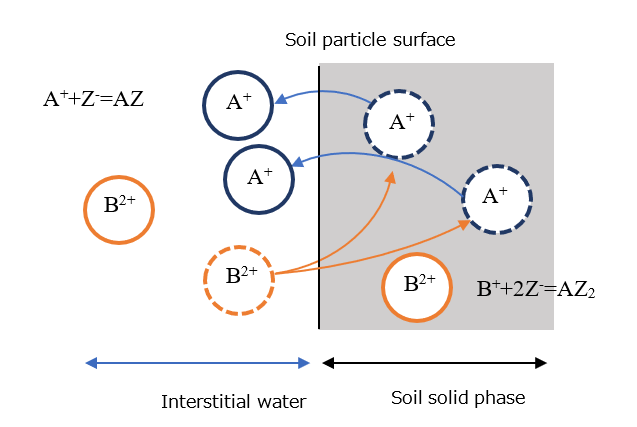
Heat Exchange between Water Flows and Solid Rock Phases
The transient behavior of high temperature groundwater, which moves in fissures and undergoes heat exchange with the surrounding rock until both reach the same temperature as time passes, is formulated as a non-equilibrium heat exchange phenomenon via the contact interface between the fluid phase and solid rock phase (Tosaka 1999). The fluid phase is treated as a mixed fluid of water and air, and the fluid phase temperature \(T_{f}\) and solid phase temperature \(T_{s}\) are used for both water and air.
Because the thermal conductivity in the solid rock phase is described in the same form as the diffusion equations previously calculated for other interphase transport phenomena, the amount of heat transfer per unit time can be expressed as follows.
\[E_{f \rightarrow s} = 2A_{\text{fs}}\sqrt{\frac{{{\lambda_{s}\rho}_{s}C}_{s}}{\pi\Delta t}}\left( T_{f} - T_{s} \right)\qquad{(4.30)}\]
In the equation, the symbols have the following meanings.
| \(C_{s}\) | Specific heat capacity of the solid phase \(\lbrack J/(K kg)\rbrack\) |
| \(A_{\text{fs}}\) | Contact area between the fluid and solid phases |
| \(\rho_{s}\) | Density of the solid phase \(\lbrack kg/m^{3}\rbrack\) |
| \(\lambda_{s}\) | Thermal conductivity of the solid phase \(\lbrack J/(K m s)\rbrack\) |
If we consider a parallel-plate-type fissure in the bed rock, then the contact area between the fluid and solid phases is given with the direction attached, as shown in Fig. 4.4 The variables \(\Delta x\), \(\Delta y\), and \(\Delta z\) in the figure are the widths of the calculation grid cell assigned to the fissure.

Physical Properties of Fluids and Geological Strata
Geofluid simulations require values related to numerous physical properties for fluids and geological strata. These values appear in the governing equations. Some of these values are constant, but many are functions of characteristics such as pressure, saturation, temperature, and density. Some functions express a simple linear relation, while others are nonlinear curves found through experimentation.
This chapter provides details regarding the fluid and strata properties handled by GETFLOWS.
Physical Properties of Fluids
Estimation of Density of Liquids and Gases
Density approximation
The following equations are the simplest forms for determining liquid and gas densities in a hydrological environment.
\[\rho_{\text{wR}} = \rho_{\text{wS}}\left( 1 + c_{w}\left( P - P_{s} \right) \right)(1 + \mathrm{\beta}{(T - T}_{S}))\qquad{(5.1)}\] \[\rho_{\text{gR}} = \frac{\rho_{\text{gS}}T_{s}P}{TP_{s}}\qquad{(5.2)}\]
Equ. 5.1 is an approximation that assumes certain coefficients of volume compression and thermal expansion for pressure and temperature within a certain range, and is applied to aqueous or non-aqueous phase liquids, such as oil or chlorinated organic solvents, respectively. Equ. 5.2 considers gases as ideal gases, and can be applied to gases at near-normal atmospheric conditions.
Water simulations can be performed for areas ranging from deep underground to high mountainous regions, so simulations of isothermal conditions require specification of typical temperatures. Normally, however, this value can be set to around 20 °C without negative impact.
For application to a broader range of pressures and temperatures, or when the presence of dissolved elements is to be considered, the following items should be kept in mind.
Formation volume factor
The formation volume factor is one method of representing density, and is often used in reservoir engineering. GETFLOWS typically uses this too, and so we explain the concept here.
Formation volume factor extracts the subsurface flow of a liquid \(V_{pR}\) and represents the flow as a ratio of the volume under standard above-ground conditions \(V_{\text{pS}}\). Letting \(\left( P_{\text{pS}},T_{\text{atm}} \right)\) and \(\left( P_{\text{pR}},T_{R} \right)\), respectively, be surface and subsurface pressure and temperature, we define the following equation.
\[B_{p} = \frac{V_{pR}\left( P_{\text{pR}},T_{R} \right)}{V_{\text{pS}}\left( P_{\text{pS}},T_{\text{atm}} \right)},\ \ p = w,g,n.\qquad{(5.3)}\]
By characterizing the differences in change in volume by temperature and pressure, we obtain the following volume coefficient.
\[B_{p} = \frac{V_{pR}\left( P_{\text{pR}},T_{R} \right)}{V_{\text{pO}}\left( P_{\text{pR}},T_{\text{atm}} \right)} \bullet \frac{V_{\text{pO}}\left( P_{\text{pR}},T_{\text{atm}} \right)}{V_{\text{pS}}\left( P_{\text{pS}},T_{\text{atm}} \right)} = B_{P}\left( P_{\text{pR}} \right) \bullet B_{T}\left( T_{R} \right)\text{.\ \ \ }\qquad{(5.4)}\]
Here, \(B_{p}\) and \(B_{T}\) are functions of pressure and temperature, respectively, represented as the change in volume \(B_{P}\left( P_{\text{pR}} \right)\) that occurs when pressure is removed by bringing the fluid to the surface while holding the subsurface temperature constant, and by the change in volume \(B_{T}\left( T_{R} \right)\) that occurs when pressure is held constant while returning only the temperature to normal conditions. The density at a given pressure and temperature can be represented by the following equation, which uses the standard density and volume coefficient.
\[\rho_{p} = \rho_{pS}\frac{1}{B_{p}}\text{\ \ }\qquad{(5.5)}\]
GETFLOWS can be provided with an arbitrary function for the volume coefficient at a specified pressure and temperature. The default values for water and NAPLs are the following linear relations.
\[B_{P}\left( P_{\text{pR}} \right) = 1 - c_{p}\left( P - P_{\text{pS}} \right),\ \ p = w,n\qquad{(5.6)}\] \[B_{\text{Tf}}\left( T_{R} \right) = 1 + \beta_{\text{Tf}}\left( T_{R} - T_{\text{atm}} \right),\ \ \ \ \ \ \ \ \ \ \ \ \ \ p = w,n\qquad{(5.7)}\]
Here, \(c_{p}\) is the water or NAPL phase volumetric compression ratio\(\lbrack\text{Pa}^{- 1}\rbrack\), and \(\beta_{\text{Tf}}\) is the heat expansion ratio\(\lbrack K^{- 1}\rbrack\). Volumetric variation of air phase is strongly affected by pressure and temperature, so assumptions of a linear relation, like those in the above equations, clearly do not hold. Instead, the following relation from the ideal gas law is used.
\[B_{g} = B_{P}\left( P_{\text{pR}} \right) \bullet B_{T}\left( T_{R} \right) = \frac{P_{\text{gS}}}{P_{\text{gR}}} \bullet \frac{T_{R}}{T_{\text{atm}}}\qquad{(5.8)}\]
In the general case of isothermal conditions, \(T_{R} = T_{\text{atm}}\) is used, allowing the equation to calculated with \(B_{T}\left( T_{R} \right)\) as 1. The densities of fluids (water or NAPLs) and gases (air or natural gas) at subsurface pressures and temperatures are calculated by dividing by the volume coefficient of the density of each fluid phase under standard conditions (1 atm, \(\ T_{s} = 20\ \)). GETFLOWS provides subsurface fluid densities in the following forms, which take into account any material components in the liquid or gaseous phases.
\[\rho_{\text{wR}} = \frac{\rho_{\text{wS}} + \sum_{}^{}{\rho_{cS,i}R_{w,i}}}{B_{w}}\qquad{(5.9)}\] \[\rho_{\text{gR}} = \frac{\rho_{\text{gS}} + \sum_{}^{}{\rho_{cS,i}R_{g,i}}}{B_{g}}\qquad{(5.10)}\] \[\rho_{\text{nR}} = \frac{\rho_{\text{nS}}}{B_{n}}\qquad{(5.11)}\]
Here, the summation is to account for material components included in the liquid or gaseous phases, and \(\rho_{cS,i}\) is the density of component i under standard conditions. Fluid densities under standard conditions are input into GETFLOWS, and the simulation evaluates the subsurface density after finding the volume coefficients for pressure and temperature, which can change from moment to moment. Note that the densities of solid mediums must take into account the adsorption–desorption of dissolved substances and the thermal conductivity of the solid phase medium. Except in special cases, the simulator internally treats these values as constants.
Viscosity Coefficient
The viscosity coefficient of fluids does not exhibit large changes with pressure, but, as with volume coefficients, this value can be represented as a function of pressure and temperature.
\[\mu_{pR} = \mu_{\text{pS}} \bullet \mu_{P}\left( P_{\text{pR}} \right) \bullet \mu_{T}\left( T_{R} \right)\text{\ \ \ }\qquad{(5.12)}\]
Here, \(\mu_{\text{pS}}\) and \(\mu_{pR}\) are, respectively, the viscosity coefficient \(\lbrack Pa s\rbrack\) under standard conditions \(\left( P_{\text{pS}},T_{S} \right)\) and under subsurface conditions \(\left( P_{\text{pR}},T_{R} \right)\). In cases where material components exist in the aqueous or gaseous phases, the viscosity coefficient between pure fluid phases is supplemented by the contribution of the material components, and represented by the following equations.
\[\mu_{wS} = \left( \mu_{\text{wS}} \right)_{0} + \ \sum_{}^{}{\mu_{cS,i}R_{w,i}}\text{\ \ }\qquad{(5.13)}\] \[\mu_{gS} = \left( \mu_{\text{gS}} \right)_{0} + \ \sum_{}^{}{\mu_{cS,i}R_{g,i}}\text{\ \ }\qquad{(5.14)}\] \[\mu_{nS} = \left( \mu_{\text{nS}} \right)_{0}\qquad{(5.15)}\]
Here, \(\left( \mu_{pS} \right)_{0}\) is the viscosity coefficient between pure fluid phases, and \(\mu_{cS,i}\) is the viscosity coefficient for component i under standard conditions. Variables \(\mu_{p}\) and \(\mu_{T}\) are, respectively, the pressure and temperature functions.
The term \(\mu_{P}\left( P_{\text{pR}} \right)\) represents the change in the viscosity coefficient when pressure is removed by bringing the fluid to the surface while holding the subsurface temperature constant, and \(\mu_{T}\left( T_{R} \right)\) is the change in the viscosity coefficient that occurs when pressure is held constant while returning only the temperature to normal conditions. There are cases where NAPLs at high temperatures or pressures can contain dissolved gas components, but such cases are not treated here.
Viscosity coefficients can be specified as functions of pressure and temperature. Under standard conditions, only the relation between viscosity coefficients and change in pressure is defined, using the following linear equation for viscosity between liquid phases.
\[\mu_{P}\left( P_{\text{pR}} \right) = 1 + c_{\mu}\left( P_{\text{pR}} - P_{\text{pS}} \right),\ \ p = w,g,n\qquad{(5.16)}\]
Here, \(c_{\mu}\) is the increase in viscosity \(\lbrack\text{Pa}^{- 1}\rbrack\) due to change in pressure, and different values can be given for each liquid phase.
Viscosity coefficients that reflect temperature change differ between liquid (water, NAPL) phases and air phases. GETFLOWS represents these by the following empirical formulas.
Liquid phase \[\mu_{T}\left( T_{R} \right) = A \bullet exp\left( \frac{B}{T_{R}} \right)\qquad{(5.17)}\]
Air phase \[\mu_{T}\left( T_{R} \right) = \left( \mu_{\text{wS}} \right)_{0}\left( \frac{T_{\text{atm}} + C}{T_{R} + C} \right)\left( \frac{T_{R}}{T_{\text{atm}}} \right)^{3/2}\qquad{(5.18)}\]
The dependence of liquid phase viscosity on temperature is described by Andrade’s equation, which is established as valid over a temperature range from near the freezing point up to the boiling point of the liquid under standard conditions. Values A and B are empirically determined constants that vary by fluid. The air phase, too, includes a constant C (Sutherland’s constant) that varies by gas; C is 117 for air. The viscosity coefficient under standard conditions is taken to be 18.2 × 10⁻⁶\(\ \text{Pa} s\).
For a wider range of temperature and pressure conditions, the international interpolation formula obtained from the steam table is used. The international interpolation formula for saturated water with a temperature range of 0–300°C is expressed by the following formula.
\[\mu_{T}\left( T_{R} \right) = 241.4 \times 10^{247.8\left\lbrack \left( T_{\text{pR}} - 140 \right) \right\rbrack^{- 1}}\qquad{(5.19)}\]
For compressed water with a temperature range of 0–300 °C and a pressure range of –800 \(\text{bar}\), the following international interpolation formula is used.
\[\mu_{pR}\left( P_{R},T_{R} \right) = 241.4 \times 10^{247.8\left\lbrack \left( T_{\text{pR}} - 140 \right)^{- 1} \right\rbrack}\qquad{(5.20)}\]
\[\left\lbrack 1 + \frac{P_{\text{pR}} - P_{\text{ps}}}{10^{6}} \bullet 1.0467\left( T_{\text{pR}} - 305 \right) \right\rbrack\]
In this international interpolation formula, the unit of viscosity coefficient is \(mP\) (micropoise), and the unit of pressure is \(\text{bar}\).
Specific Heat Capacity
Specific heat at constant pressure for water and air phases is defined by the following equation.
\[c_{p} = \left( \frac{\partial H}{\partial T} \right)_{p = const.}\qquad{(5.21)}\]
When pressure is held constant, the change in total heat equals the change in enthalpy. When volume is held constant, the change in total heat equals the change in internal energy.
The specific heat of the water phase is interpolated from steam tables, which account for dependence on pressure and temperature. GETFLOWS contains specific heat for temperatures in the range 0–260 °C and pressures in the range 0.1–100 atm.
| Substance | Temp [°C] | Specific heat [kJ/(kg·°C)] |
|---|---|---|
| Gases | Air | 50 (20 atm) |
| Water vapor | 100 | |
| Oxygen | 15 | |
| Methane | 15 | |
| Metals | Aluminum | 20 |
| Cast iron | 20–100 | |
| Copper | 15–100 | |
| Inorganic compounds | Calcium carbonate | 0 |
| Calcium sulfate | 36 | |
| Organic compounds | Benzene | 20 |
| Ethyl alcohol | 25 | |
| Dry rock | Basalt | 20–100 |
| Chalk | 20–100 | |
| Claystone | 20–100 | |
| Granite | 12–100 | |
| Quartz | 12–100 |
Saturated Vapor Pressure
Saturated water vapor pressure is a function of temperature and is calculated with the surface tension effects of water droplets taken into account. The Kelvin equation shown below is used.
\[P_{\text{sat}}\left( S_{w},T \right) = P_{\text{sat}}\left( T \right) \bullet exp\left\lbrack \frac{M_{w}P_{c,w}\left( S_{w} \right)}{\rho_{w}\text{RT}} \right\rbrack\qquad{(5.22)}\]
Here, \(M_{w}\) is molecular weight, \(P_{c,w}\left( S_{w} \right)\) is the capillary pressure force \(\lbrack Pa\rbrack\) between water and air phases, obtained as a function of the water phase saturation, and \(R\) is a gas constant\(\lbrack J/(K kg)\rbrack\).
Physical Properties of Porous Media
Porosity
Geology and porosity ratio
There are two types of porosity values: those obtained by dividing the total porosity volume of the medium by the bulk volume of the sample (the absolute porosity), and those obtained by isolating the porosity in the medium (the effective porosity). The absolute and effective porosities are obtained in roughly the following ranges.
| Medium | Absolute porosity | Effective porosity | Notes |
|---|---|---|---|
| Soil | 80–50% | Approx. same | Effective porosity is slightly smaller |
| Gravel | 40–20% | Approx. same | Effective porosity is slightly smaller |
| Mudstone | Approx. 40% | Differs by a few % | Many isolated voids due to small particles and compaction solidification |
| Limestone | Approx. several percent to 10% | Approx. same | Due mainly to vugs |
| Granite | Approx. several percent | Differs by a few percent | Due mainly to cracks |
Simulations consider mainly voids as contributing to flow, so the effective porosity is input. Note that this input must consider the strong correlation between the porosity value and permeability.
Changes in porosity due to pore pressure
Porosity can vary due to variation in air and hydraulic pressure within voids. Such variation will be small in strata with high agglomeration, and large in near-surface strata with low agglomeration. Generally, the following first-order approximation is used, under the assumption that void deformation occurs due to micro-elasticity (this is in the same form as the first-order approximation for variation in water density).
\[\phi = \phi_{0}\left( 1 + c_{\phi}\left( P - P_{s} \right) \right)(1 + \mathrm{\beta}_{\phi}{(T - T}_{S}))\qquad{(5.23)}\]
Here, \(\phi\) is the porosity of the medium for a given pressure and temperature\(\lbrack - \rbrack\), \(\phi_{0}\) is the porosity under standard conditions, \(P\) is the fluid pressure \(\lbrack\text{Pa}\rbrack\) in pores, \(c_{\phi}\) is the volume compression ratio \(\lbrack\text{Pa}^{- 1}\rbrack\) in pores, \(\beta_{\phi}\) is the thermal expansion ratio \(\lbrack C^{- 1}\rbrack\), \(T_{s}\) is the reference temperature, and \(P_{S},\ T_{S}\) are respectively the air pressure \(\lbrack Pa\rbrack\) and temperature [°C] under standard conditions. The change in only pressure is considered under isothermal conditions.
Note that the combined compression ratios of water and the medium are referred to as the combined compression ratio, and the product of this and the porosity under the reference conditions is called the specific storage (Tosaka 2006).
Large pore deformation
In cases where fluids in strata result in extremely large pore pressures, a linear relation that assumes micro-deformations no longer holds. For this reason, GETFLOWS allows selection of the following structural model, which considers stress dependence of the effective porosity (Gangi 1978).
\[\phi = \phi_{0}\left\lbrack 1 - \left\{ \frac{\sigma - P_{\text{fR}} - \beta_{\text{Ts}}E\left( T_{s} - T_{\text{atm}} \right)}{P_{x}} \right\}^{m} \right\rbrack\qquad{(5.24)}\]
Here, \(\sigma\) is the rock stress (assuming isotropy), E is Young’s modulus, and \(P_{x},\ m\) are empirical constants, which must be established for the specific site. In this equation, \(\sigma - P_{\text{sR}} - \beta_{\text{Ts}}E\left( T_{s} - T_{\text{atm}} \right)\) represents the effective stress.
Flow channel widening that results from pore pressure exceeding a certain threshold is represented by the following bilinear equations.
\(P_{\text{fR}} \leq P_{1}\) ; \[\phi = \phi_{0}\left\{ 1 + c_{s}\left( P_{\text{fR}} - P_{0} \right) \right\}\qquad{(5.25)}\] \(P_{\text{fR}} > P_{1}\) ; \[\phi = \phi_{0}\left\lbrack 1 - c_{s}\left( P_{1} - P_{0} \right) + {F \bullet c}_{s}\left( P_{\text{fR}} - P_{1} \right) \right\rbrack\qquad{(5.26)}\]
Here, \(P_{1}\) is the pressure threshold \(\lbrack Pa\rbrack\) that results in channel widening, and F is an empirical constant.
Absolute Permeability
Hydraulic conductivity and permeability
Hydraulic conductivity and permeability for saturated groundwater flow are given by the following relation.
\[k = \frac{\rho\text{gK}}{\mu} = \frac{10^{3} \times 9.8 \times K}{10^{- 3}} \approx 10^{7}K\qquad{(5.27)}\]
Here, \(k\ \lbrack m/s\rbrack\) is the saturated hydraulic conductivity, and K is the absolute permeability \(\lbrack m^{2}\rbrack\). Absolute permeability is specific to the physical properties of the porous medium, and saturated hydraulic conductivity is a mixed parameter of the fluid and medium properties. The relation between the two is given by the above equation, but a typical example is \(10^{- 5}\ m/s \approx 10^{- 12}\ m^{2}\).
In groundwater analysis, the saturated hydraulic conductivity is often simply called the “permeability coefficient” but generalized multi-phase flow analysis uses absolute permeability. See (Tosaka 2006) for the permeability values of a variety of substances.
There is anisotropy in the strata permeability values; in particular there are significantly different values between horizontal and vertical directions. In actual value calculations, these values are the most dominant factors affecting groundwater flow, but since it is impossible to provide clear values over all ranges, absolute permeability is entered according to the geological distribution (lithology distribution) over the grid or region.
Relation with effective porosity
The spaces between strata are thought to undergo micro-deformations due to hydraulic pressure. Specifically, when hydraulic pressure decreases, the pores slightly contract, with changes permeability. Such variation can be modeled by a structural relation between the effective porosity and absolute permeability, as follows.
\[K = \text{aK}_{0}\left( \frac{\phi}{\phi_{0}} \right)^{m}\qquad{(5.28)}\]
Here, \(K_{0}\) is the initial absolute permeability \(\lbrack m^{2}\rbrack\) under standard conditions, and a and m are empirical constants.
Gas permeability
The basis for multi-phase flow formulation is generally an equivalence between the values for absolute permeability obtained through saturated permeability testing and the values for absolute permeability obtained through air permeability testing, but these values can differ under specific circumstances. For a nonzero flow due to slip effects (free flow of gas molecules) in the vicinity of void walls, gas permeability is given by the following equation (Klinkenberg 1941).
\[K_{g} = K_{w}\left( 1 + \frac{b}{P_{\text{gR}}} \right)\qquad{(5.29)}\]
Here, b is the Klinkenberg parameter \(\lbrack Pa\rbrack\), and \(P_{\text{gR}}\) is the gas pressure under subsurface conditions. This pressure is determined by the magnitude relation between the size of the pores forming the flow path and the mean free path of the gas molecules. When \(P_{\text{gR}}\) is large, there is a reduced slip effect, and the absolute permeabilities of the air and liquid phases will be consistent.
The Klinkenberg parameter varies according to the medium, gas type, and temperature. For air, the following relational equations have been proposed for use in determining gas permeability.
(Thorstenson 1989) \[b = 0.11{K_{w}}^{- 0.39}\qquad{(5.30)}\] (Jones 1980) \[b = 0.98{K_{w}}^{- 0.33}\qquad{(5.31)}\]
Equ. 5.30 is a correlation equation estimated from samples with permeability in the range \(10^{- 12} - 10^{- 17}\ m^{2}\). Equation Equ. 5.31 is a correlation equation estimated from samples with permeability in the range \(10^{- 14} - 10^{- 19}\ m^{2}\). From these equations, the Klinkenberg parameter takes the range \(10^{3} - 10^{6}\).
Capillary Pressure
Multi-phase flow simulations of water, air, and NAPLs must evaluate capillary pressure caused by the interfacial effects between different fluid phases.
When fluids in three phases coexist, GETFLOWS always treats water phases as wetting phases and air phases as non-wetting phases2.
The pressure of water and air phases is evaluated by using the capillary force resulting between NAPL phases according to the following relations.
\[P_{w}\left( S_{w} \right) = P_{n} - P_{c,wn}\left( S_{w} \right)\qquad{(5.32)}\] \[P_{g}\left( S_{g} \right) = P_{n} + P_{c,gn}\left( S_{g} \right)\qquad{(5.33)}\]
Note that the capillary force between air and NAPL phases is considered to be 0. In typical situations, such as shallow groundwater, where there is an (unsaturated) water phase and an air phase, the water phase is the wetting phase and the air phase is the non-wetting phase. The fluid phase pressure is therefore calculated from the capillary force of both phases by the following equation.
\[P_{w}\left( S_{w} \right) = P_{g} + P_{c,wg}\left( S_{w} \right)\qquad{(5.34)}\]
For the specific capillary force, the effective saturation level \(S_{e}\) is defined as a nonlinear function by the following equation.
\[S_{e} = \frac{S_{w} - S_{\text{wr}}}{1 - S_{\text{wr}}}\qquad{(5.35)}\]
Here, \(S_{\text{wr}}\) is the residual water saturation of the water phase. In GETFLOWS, the relation between capillary pressure and water phase saturation can be input as values in a discrete value table. A given water phase saturation that changes with time is calculated by using capillary pressure as linearly interpolated from the input table values. Some frequently used capillary pressure models are stored as function formulas and can be used by providing the appropriate parameters.
The van Genuchten model
The van Genuchten model uses the effective saturation level \(S_{e}\) as defined by the above equation to determine the capillary force at a given saturation by the following equation.
\[P_{c} = \frac{1}{\alpha}\left( S_{e}^{- \frac{1}{m}} - 1 \right)^{\frac{1}{n}}\qquad{(5.36)}\]
Here, \(\alpha\) is a parameter related to the capillary force, and \(\text{m\ }\) and \(n\) are empirical parameters. When measurement data resulting from laboratory core sample testing are available, these are used along with a fitting parameter applied to the input data. Normally, the relation \(m = 1 - 1/n\) will hold.
The Brooks–Corey model
As with the van Genuchten model, the Brooks–Corey model defines a relation with effective saturation. In the model, this is given as follows.
\[P_{c} = p_{d}S_{e}^{- \frac{1}{\lambda}}\qquad{(5.37)}\]
Here, \(\lambda\) is a shape parameter that characterizes the pores, found as the slope of a log–log plot of the relation between capillary pressure and saturation. This is also referred to by terms such as the pore size index. The intrusion pressure required for the non-wetting phase fluid (the air phase) to displace the wetting phase fluid (the water phase in the case of a water–air two-phase system) is \(p_{d}\). This is also called the bubbling pressure or the displacement pressure.
Relative Permeability
The relative permeability in a two-phase system (e.g., NAPL–water, air–NAPL, air–water) considers the displacement process of the two fluid phases, which is described by increasing or decreasing the saturation of the fluid phase in only one of the fluid systems that does not consider hysteresis.
Unsaturated relative permeability, which is important in the analysis of water circulation systems, is evaluated according to the relative permeability curve used in the water–air two-phase flow model, but there are only limited situations in which per-strata measurement data can be obtained. In practice, it is typical to use an empirical formula obtained from experiments on similar soil samples, or a relational expression giving only general trends. In cases where good measurement data can be obtained on-site or in the lab, indirect identification through inverse analysis is often performed.
Multi-phase simulations have long been practically applied to areas of petroleum engineering that are concerned with oil and gas fields because empirical formulas derived from experiments using rock samples can be used. Also, such empirical formulas are often applied to more general cases of groundwater analysis in conjunction with experimental parameters related to rock samples having similar properties. GETFLOWS comes with several typical permeability models that users can specify and use by providing experimentally obtained parameter values. Additionally, by supplying a table that describes the relation between saturation and relative permeability, a desired relative permeability model can be incorporated into simulations.
Considering the general state of two coexisting water and air phases, and taking the water phase as the wetting phase and the air phase as the non-wetting phase, the following empirical relations can be used with the respective relative permeability curves.
The Corey model
The Corey model describes the relative permeability curve of the water and gas phases as the following power law for the effective saturation:
\[k_{\text{rw}} = S_{e}^{4}\qquad{(5.38)}\] \[k_{\text{rg}} = \left( 1 - S_{e} \right)^{2}\left( 1 - S_{e}^{2} \right)\qquad{(5.39)}\]
The definition of effective saturation is the same as Equ. 5.35 used in the functional equation for the capillary pressure curve. This does not include parameters for media-specific pore characteristics; thus, the Brooks–Corey model is often used when fitting of experimental data is to be performed.
The Brooks–Corey model
The Brooks–Corey model is described by the following relations, which consider the pore form parameter \(\lambda\).
\[k_{\text{rw}} = S_{e}^{\frac{2 + 3\lambda}{\lambda}}\qquad{(5.40)}\] \[k_{\text{rg}} = \left( 1 - S_{e} \right)^{2}\left( 1 - S_{e}^{\frac{2 + \lambda}{\lambda}} \right)\qquad{(5.41)}\]
The van Genuchten model
The van Genuchten model is one of the most commonly used models, and is represented by the following equations. The empirical parameters \(m,n\) are the same as those in the capillary pressure curve of Equation (XX).
\[k_{\text{rw}} = S_{e}^{\varepsilon}\left( 1 - \left( 1 - S_{e}^{\frac{1}{m}} \right)^{m} \right)^{2}\qquad{(5.42)}\] \[{k_{\text{rg}} = \left( 1 - S_{e} \right)^{\gamma}\left( 1 - S_{e}^{\frac{1}{m}} \right)}^{2m}\qquad{(5.43)}\]
Here, \(\varepsilon = 1/2,\gamma = 1/3\), and these empirical parameters reflect the connections between pore structures. The relative permeability of the non-wetting phase (the air phase) was expanded by Parker (1987) and Luckner (1989) to obtain a general form of the above equations.
The Grant model
In cracks and fissures in a medium, there is little inter-phase interference between the wetting- and non-wetting phases, and it has been experimentally established that the following linear relation holds for the relative permeability curve between wetting- and non-wetting phases .
\[k_{\text{rw}} + k_{\text{rg}} = 1\qquad{(5.44)}\]
This relation has been used in many reservoir simulations, but numerous other proposals have been made regarding dual phases in cracks and fissures. The following relations, which apply the Corey model to the wetting phase and the Grant model to the non-wetting phase, are included for use in general-purpose numeric simulations of multi-phase, multi-component flow .
\[k_{\text{rw}} = S_{e}^{4}\qquad{(5.45)}\] \[k_{\text{rg}} = 1 - k_{\text{rw}}\qquad{(5.46)}\]
Relative permeability in a 3-phase system
GETFLOWS allows the arbitrary specification of combined permeability models to be applied to wetting- and non-wetting phases, so selection can be performed as appropriate for the characteristics of the rock solid and fluid phases in question. In situations where water, air, and NAPL phases coexist, a three-phase relative permeability is commonly calculated from the two-phase permeabilities, for example those between the air and water phases and between the air and NAPL phases.
GETFLOWS uses the following representative methods.
The Stone primary method
The Stone secondary method
The saturation-weighted interpolation method
The Parker method
These methods make the following assumptions regarding the wetting properties of the three fluid phases with respect to filling of pores (Tosaka 2006).
So long as the water phase is the wetting phase for solid particles, water works on only the solid side, and fluid on the pore side is not dependent on the gas or NAPL. The relative permeability of water is determined solely by the degree of water saturation. Liquids easily separate gases from solids and exist in the most interior part of pores, and external fluids move with almost no effect by water or NAPLs. The relative permeability of gases is determined solely by the degree of gas saturation.
NAPLs, which are an intermediary phase between wetting and non-wetting phases, come into contact with gases and water, and movement is reliant on the degree of saturation of both. The relative permeability of NAPLs is a function of the saturation of both the gaseous and water phases.
The Stone primary method
\[k_{\text{rn}} = \frac{S_{\text{ne}}k_{rn(w)}k_{rn(g)}}{k_{rn(w)}\left( 1 - S_{\text{we}} \right)\left( 1 - S_{\text{ge}} \right)}\qquad{(5.47)}\] \[S_{\text{ne}} = \frac{S_{n} - S_{\text{nm}}}{1 - S_{w,irr} - S_{n,irr}}\qquad{(5.48)}\] \[S_{\text{we}} = \frac{S_{w} - S_{w,irr}}{1 - S_{w,irr} - S_{n,irr}}\qquad{(5.49)}\] \[S_{\text{ge}} = \frac{S_{g}}{1 - S_{w,irr} - S_{\text{nm}}}\qquad{(5.50)}\] \[S_{\text{nm}} = \lambda S_{w,irr} + \left( 1 - \lambda \right)S_{n,irr}\qquad{(5.51)}\] \[\lambda = 1 - \frac{S_{g}}{1 - S_{w,irr} - S_{n,irr}}\qquad{(5.52)}\]
The Stone secondary method
\[k_{\text{rn}} = \left( k_{\text{rn}\left( w \right)} + k_{\text{rn}\left( w,irr \right)}k_{\text{rw}\left( n \right)} \right)\left( k_{\text{rn}\left( g \right)} + k_{\text{rn}\left( w,irr \right)}k_{\text{rg}\left( n \right)} \right)\qquad{(5.53)}\]
\[- k_{rn(w,irr)}\left( k_{rw(n)} + k_{rg(n)} \right)\]
The saturation-weighted interpolation method
\[k_{\text{rn}} = \frac{\left( S_{w} - S_{w,irr} \right)k_{\text{rn}\left( w \right)} + \left( S_{g} - S_{g,irr} \right)k_{\text{rn}\left( g \right)}}{\left( S_{w} - S_{w,irr} \right) + \left( S_{g} - S_{g,irr} \right)}\qquad{(5.54)}\] \[k_{\text{rw}} = \frac{\left( S_{n} - S_{n,irr} \right)k_{\text{rw}\left( n \right)} + \left( S_{g} - S_{g,irr} \right)k_{\text{rn}\left( g \right)}}{\left( S_{n} - S_{n,irr} \right) + \left( S_{g} - S_{g,irr} \right)}\qquad{(5.55)}\] \[k_{\text{rg}} = \frac{\left( S_{w} - S_{w,irr} \right)k_{\text{rn}\left( w \right)} + \left( S_{n} - S_{n,irr} \right)k_{\text{rg}\left( n \right)}}{\left( S_{w} - S_{w,irr} \right) + \left( S_{n} - S_{n,irr} \right)}\qquad{(5.56)}\]
The Parker method
\[k_{\text{rn}} = \left\lbrack \frac{S_{n}}{1 - S_{w,irr}} \right\rbrack^{\frac{1}{2}}\left\lbrack \left( 1 - {S_{w}}^{\frac{n}{n - 1}} \right)^{\frac{n - 1}{n}} - \left( 1 - {S_{t}}^{\frac{n}{n - 1}} \right)^{\frac{n - 1}{n}} \right\rbrack^{2}\qquad{(5.57)}\] \[S_{t} = \frac{S_{n} + S_{w} + S_{w,irr}}{1 - S_{w,irr}}\qquad{(5.58)}\]
Here, \(k_{rp}\) is the relative permeability and \(S_{p}\) is the saturation. The subscript p indicates the phase (g for gaseous, w for water, n for NAPL), and \(S_{p,irr}\) is the residual saturation for fluid phase p. Subscripts in parentheses on relative permeabilities indicate fluid phases.
Hysteresis
This section will be completed in a forthcoming update.
Pore Tortuosity
Tortuosity in highly porous media is represented as \(\tau = S/L\) for a flow path of substantial length \(S\) over which the flow is linearly cross-section separated by \(L\). This is used when mass transfer due to diffusion in the medium is considered, and various representations of its relation with porosity are used. GETFLOWS allows arbitrary specification of tortuosity for each region by computational grid or stratum section. GETFLOWS provides the following relational equation, which is from a structural model derived from a theoretical investigation of pore distributions (Millington 1961) and has been expanded to multi-phase systems.
\[\tau = \tau_{0}\tau_{s} = \phi^{\frac{1}{3}}{S_{p}}^{\frac{7}{3}}\qquad{(5.59)}\]
Here, \(\tau_{0}\) is the degree of tortuosity \(\lbrack - \rbrack\) due to structural factors of the medium, and \(\tau_{s}\) is the degree of tortuosity \(\lbrack - \rbrack\) due to the mixture of multiple fluids in pores. The residual fluid distribution in pores, as represented by the residual saturation, is considered as not contributing to flow path connectedness, so \(S_{p} = S_{p} - S_{p,irr}\), where \(S_{p,irr}\) is the residual saturation of fluid phase p.
Diffusion Coefficient
Molecular diffusion
Molecular diffusion of dilute solute concentration in water phases is calculated according to the following equation, which considers and adjusts for temperature, pressure, and changes in viscosity (Reid 1987).
\[D_{w,i} = \left( D_{w,i} \right)_{0}\frac{T_{\text{wR}}}{T_{\text{atm}}}\frac{\mu_{\text{wS}}}{\mu_{wR}}\qquad{(5.60)}\]
Here, \(\left( D_{w,i} \right)_{0}\) is the molecular diffusion coefficient of solute i under normal conditions, found by the widely used correlation equation from Wilke and Chang (1955).
\[\left( D_{w,i} \right)_{0} = \frac{7.4 \times 10^{- 8}\left( \psi_{w}M_{w,i} \right)^{1/2}T_{\text{wR}}}{\mu_{wR}{V_{w,i}}^{0.6}}\qquad{(5.61)}\]
Here, \(\psi_{w}\) is the dimensionless solute association factor, which in the case of the water phase is 2.6. \(M_{w,i}\) and \(\ V_{w,i}\) are respectively the molecular weight [g/mol] and molar volume [cm3/mol] of solute i.
The molecular diffusion coefficient for a gaseous component i in an air phase is calculated in consideration of its dependence on temperature and pressure according to the following empirical equation.
\[D_{g,i} = \left( D_{g,i} \right)_{0}\frac{P_{\text{atm}}}{P_{gR}}\left( \frac{T_{\text{fR}}}{T_{\text{atm}}} \right)^{n}\qquad{(5.62)}\]
Here, \(\left( D_{g,i} \right)_{0}\) is the molecular diffusion coefficient under standard conditions. The value of n will vary by gas components but typical values are 1.67 for oxygen and hydrogen and 1.71 for carbon dioxide.
Note that the current version of GETFLOWS does not consider molecular diffusion of solutes in NAPLs.
Effective dispersion
Dispersion within geologic strata is used as an effective dispersion coefficient that considers a two-phase state and pore tortuosity for the free water and air molecular dispersion coefficient. The effective dispersion coefficient for a water- and air-phase condition containing saturated and unsaturated regions is given by the following equation.
\[\text{De}_{p,i} = \frac{D_{p,i}\phi}{\tau}G\qquad{(5.63)}\]
Here, \(\text{De}_{p,i}\) is the effective dispersion [m2/s] of solute i in phase p, and G is the ratio of the water phase in pores, calculated as follows.
\[G = \left( \frac{S_{p} - S_{p,irr}}{1 - S_{p,irr}} \right)^{n}\qquad{(5.64)}\]
Here, \(S_{w,irr}\) is the residual saturation of phase p, which considers residual fluid in pores as not contributing to dispersion of solute concentration. The value of n is empirically derived.
GETFLOWS contains other structural equations for evaluating effective dispersion, as follows.
\[\text{De}_{p,i} = \tau S_{p}\phi D_{p,i}\qquad{(5.65)}\] \[\text{De}_{p,i} = aD_{p,i} \bullet exp\left( \text{bS}_{p}\phi \right)\qquad{(5.66)}\]
In Equ. 5.66, \(a,b\) are empirically derived constants that differ according to the combination of solvent and stratum medium.
The following equation calculates the turbulent diffusion coefficient for solutes and suspended sediment transported by surface water.
\[\text{De}_{w,i} = \frac{1}{6}\kappa u_{l}^{*}h\qquad{(5.67)}\]
Here, \(\kappa\) is the Kármán constant, \(u_{l}^{*}\) is the dimensionless friction velocity, and h is the water flow depth.
Thermal Conductivity
The description of flow under non-isothermal conditions is performed by simultaneously solving the energy and mass conservation equations. To do so, GETFLOWS evaluates the thermal conductivity of liquid, gas, and solid phases. Internally, the simulator uses the thermal conductivity of water and air phases, handling the mean values of each according to their relative abundance. Specifically,
\[K_{T,f} = K_{T,w}S_{w} + K_{T,g}\left( {1 - S}_{w} \right).\qquad{(5.68)}\]
The thermal conductivity of the water phase and air phase under a wide range of temperature and pressure conditions can be obtained by the international interpolation formula shown in the steam table. The thermal conductivity of compressed water with a temperature range of 0–350 °C and a pressure range of saturation pressure –500 bar is calculated by the following formula.
\[K_{pR}\left( P_{\text{pR}},T_{R} \right) = a_{0} + a_{1}\left( \frac{T_{\text{fR}}}{T_{\text{atm}}} \right) + a_{2}\left( \frac{T_{\text{fR}}}{T_{\text{atm}}} \right)^{2} + a_{3}\left( \frac{T_{\text{fR}}}{T_{\text{atm}}} \right)^{3} + a_{4}\left( \frac{T_{\text{fR}}}{T_{\text{atm}}} \right)^{4}\]
\[+ \left( P_{\text{pR}} - P_{s} \right)^{}\left\lbrack b_{0} + b_{1}\left( \frac{T_{\text{fR}}}{T_{\text{atm}}} \right) + b_{2}\left( \frac{T_{\text{fR}}}{T_{\text{atm}}} \right)^{2} + b_{3}\left( \frac{T_{\text{fR}}}{T_{\text{atm}}} \right)^{3} \right\rbrack\]
\[+ \left( P_{\text{pR}} - P_{s} \right)^{2}\left\lbrack c_{0} + c_{1}\left( \frac{T_{\text{fR}}}{T_{\text{atm}}} \right) + c_{2}\left( \frac{T_{\text{fR}}}{T_{\text{atm}}} \right)^{2} + c_{3}\left( \frac{T_{\text{fR}}}{T_{\text{atm}}} \right)^{3} \right\rbrack\]
\[a_{0} = - 922.47,\ \text{\ a}_{1} = 2839.5,\ \text{\ a}_{2} = - 1800.7,\ \text{\ a}_{3} = 525.77,\ a_{4} = - 73.440\]
\[b_{0} = - 0.94730,\ b_{1} = 2.5186,\ b_{2} = - 2.0012,\ \text{\ b}_{3} = 0.51536\]
\[c_{0} = 1.6563 \times 10^{- 3},\ c_{1} = - 3.8929 \times 10^{- 3},\ c_{2} = 2.9323 \times 10^{- 3},\ \text{\ c}_{3} = - 7.1693 \times 10^{- 3}\]
Here, \(P_{s}\) is the absolute pressure \(\left( \text{bar} \right)\) in the saturated state. In this international interpolation formula, the unit of thermal conductivity is \(mW/m/\), and the unit of pressure is \(\text{bar}\).
The thermal conductivity of solid phases is generalized by the following equation, which considers dependence on temperature and water phase saturation.
\[K_{T,s}\left( T_{\text{sR}},S_{w} \right) = K_{\text{ref}} \bullet K_{T}\left( T_{\text{sR}} \right) \bullet K_{\text{sw}}\left( S_{w} \right)\qquad{(5.69)}\]
Here,\(\ K_{T,s}\left( T_{\text{sR}},S_{w} \right)\) is the thermal conductivity of the solid phase, \(K_{T}\left( T_{\text{sR}} \right)\) is the thermal conductivity represented as a function of temperature, and \(K_{\text{sw}}\left( S_{w} \right)\) is the thermal conductivity of the solid phase represented as a function of water phase saturation. The relation between thermal conductivity and temperature is calculated according to the following linear relation.
\[K_{T,s}\left( T_{\text{sR}} \right) = \left\lbrack 1 + \frac{1}{K_{\text{ref}}}s_{1}\left( T_{\text{sR}} - T_{\text{ref}} \right) \right\rbrack\qquad{(5.70)}\]
Here, \(K_{\text{ref}},\ \text{\ and\ }T_{\text{ref}}\) are respectively the thermal conductivity [J/(K · m · s)] of the solid phase under standard conditions and at a given temperature [K], and \(s_{1}\) is the increase in thermal conductivity by unit temperature change (i.e., the thermal conductivity gradient). The relation between water phase saturation and temperature is given by the following formula.
\[K_{\text{sw}}\left( S_{w} \right) = \left\lbrack 1 + \frac{1}{\left( K_{T,s} \right)_{d}}s_{2}\sqrt{S_{w}} \right\rbrack\qquad{(5.71)}\]
Here, \(\left( K_{T,s} \right)_{d}\) is the thermal conductivity under absolute dry conditions, and \(s_{2}\) is the increase from absolute dry conditions by unit change in water phase saturation. The thermal conductivity under total saturation is given by \(\left( K_{T,s} \right)_{d} + s_{2}\), which is the mean thermal conductivity including the solid phase and liquid phase in pores.
Numerical Methods
Discretization of the 3D Geosphere System
GETFLOWS models overall flow using one-dimensional problems from small, laboratory-scale core samples (from above-ground atmospheric space, ground surface, subsurface areas, areas including seawater, etc.) to perform discretization based on a three-dimensional deformation structured grid.
Basic Structure
As described in Chapter 2, the following grid phases are available.
Atmospheric grid
Above-ground atmospheric grids (atmospheric boundary phases) are represented as a primary grid layer. Here, to model the physical world, the capillary pressure is 0 (free space), and because atmospheric spaces have extremely large capacity, the porosity is treated as numerically infinite, so penetration is treated as extremely high and aqueous saturation is extremely low. Flow between surface and atmospheric phase grids is calculated according to the pressure gradient. It is possible to apply a standard atmospheric pressure to the overall atmospheric grid, and to apply spatial distributions reflecting the pressure distribution on a per-grid basis. Inflow and outflow of water at the surface grid layer due to entering or leaving air are also represented.
Ground surface grid
In ground surface grids, surface water flowing in rivers or along slopes and water retention by lakes and oceans are represented. Movement of surface water is treated as Manning-type open-channel flow that follows a ground surface grid. Differences in mobility of surface water due to location are set by using roughness coefficients that depend on land use and land cover. The porosity of surface phases is normally 1.0 and capillary pressure is normally 0, but pseudo-capillary effects are calculated for underground seepage to allow consistent representation of seep and spread.
Subsurface grids
In subsurface grids, multi-phase multi-component fluid flow in subterranean media is represented in accordance with the generalized Darcy’s law. Hydraulic properties of strata (porosity, penetration rate, capillary pressure curve, relative permeability curve) are provided for each grid. Fluid pressure, saturation, temperature, concentration, and other such properties are treated as unknown quantities.
Grids representing manmade structures
Grids with large capacity, such as those for surface dams and atmospheric layers, can also be used to model boundary conditions for underground tunnels and laboratory tests. To achieve this in the case of underground tunnels, the pressure of a stratum grid corresponding to the excavation at a given time is taken as standard atmospheric pressure, a sufficiently small value is taken as saturation (for example, residual water saturation), and porosity is made sufficiently large. The state quantity of the excavation grid is not changed by fluid flowing into the grid, and incoming fluid is treated as flowing out of the system. In a similar manner, for cases such as when one end of a rock core used in laboratory testing is pressure affixed, a grid with large volume is attached to the end of the sample to simulate the operating pressure.
To represent subsurface fluids in strata representing geologic strata structures, the uppermost strata grid can be taken as a sand exchange phase, allowing landform change to be represented as erosion or deposition due to sand flow. As above, a surface fluid phase and atmospheric phase are placed above the sediment exchange phase.
The above surface fluid, atmospheric, and subsurface fluid phases can be arbitrarily specified, and any combination of grids can be taken to represent the 3D grid system of interest.
Basic unknown quantities for each grid are pressure, saturation, concentration, and temperature. In particular, when a soil exchange phase is to be considered, a grading height that reflects the results of topographic change analysis is applied, and corner-point coordinate values of the ground surface are allowed to change from moment to moment.
Spatial Discretization (Corner-point Finite-difference Grid Systems)
Spatial discretization of the target system is basically a general Cartesian grid (rectangular lattice) and irregular corner-point differential grid system. The corner-point differential grid is designed to realize spatial representations of complex terrain, geological structures, and man-made structures represented by a typical differential grid based on a structured grid system of orthogonal divisions . When large grids with local distortion are used, there is a risk of numerical instability, but in practice the errors are usually in a range that is not problematic for large-scale analysis.
Fig. 6.1 shows an overview of the grid partitioning. The general differential grid is based on orthogonal divisions, allowing use of only grid widths \(x_{i},y_{i},z_{i}\) for each three-dimensional component to easily calculate geometry data such as grid area, area shared with adjacent grids, and inter-grid distance [Reference needed]. Note, however, that spatial representations of slopes and sloping faults within geographic strata are approximated. Corner-point differential grids, in contrast, allow arbitrary positioning within a given range such that the coordinates of grid vertices do not overlap or intersect in the same grid [Reference needed].
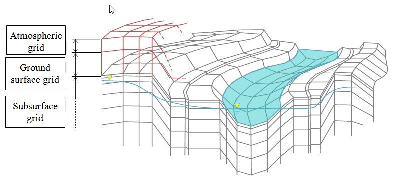
In GETFLOWS the z-direction is fixed as a vertical plane, and the elevations of corner points in the plane direction are allowed to be different. In some cases, a surface created from four points may not form a plane, so a point with the mean elevation of the four points is placed in the center, and the simulator uses this to calculate geometric form data such as surface area and center of gravity, as well as to precisely evaluate the distance between adjacent grids, surface areas, physical properties between grids and other such things. This allows flexible modeling of complex formations that would be difficult with spatial representation by normal differential grids.
GETFLOWS integrates the volume (mass) flux of each fluid phase entering and leaving each grid, and employs an integral finite-difference method that guarantees local mass balance, thereby constructing a system of equations that discretizes the entire system. Integral finite-difference methods using a corner-point difference grid can be easily applied to grid partitioning of any shape, including unstructured grid systems, and furthermore allow application of local grid-block refinement for local subdivisions of grid partitions in a given area. Evaluation of various quantities such as inter-grid penetration rates and distances for grid partitions of an arbitrary shape is heavily dependent on the adopted discrete grid form and partitioning method, so many general-purpose numeric simulators demand that users input the various values required for calculating inter-grid physical properties. In the current version of GETFLOWS, such pre-processing work is not needed because structural grid systems are limited to hexahedral grids, which allows for automatic calculation of these values within the simulator.
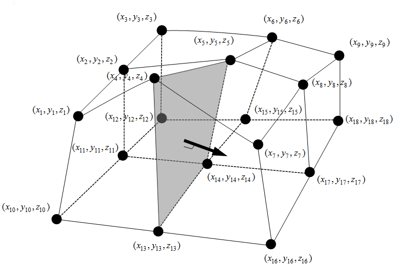
Methods for Solving Nonlinear Differential Equations
Most natural phenomena are nonlinear, with the flow of rivers and multi-phase flow being typical examples. Nonlinear problems must be solved by iterative methods, such as Newton’s method. To allow simultaneous and fully implicit solutions to problems in the case where there are multiple state quantities (unknown quantities), GETFLOWS applies Newton’s method based on a block matrix.
Newton’s Method and Difference Expansion – Representation of Temporal and Spatial Discretization
Here, we describe the method of solving for the most basic situation handled by the simulator: the case of an air–water two-phase system. Note that we use the first-order upwind difference in the space discretization of the flow term to obtain a fully implicit temporal discretization. For a hexahedral grid occupying a volume \(V_{B}\), simultaneous full implicit discretization of the fluid balance for a multi-phase, multi-component system is performed, which is shown here in residual form.
\[R_{wi} = \sum_{l = x,y,z}^{}{{A_{l}}^{n}{m_{w,l}}^{n + 1}} - {V_{B}}^{n}\left( \rho_{\text{wS}}q_{w} \right)^{n + 1}\qquad{(6.1)}\]
\[- \frac{{V_{B}}^{n}}{t}\left\lbrack \left( \frac{{\rho_{\text{wS}}\phi S}_{w}}{B_{w}} \right)^{n + 1} - \left( \frac{{\rho_{\text{wS}}\phi S}_{w}}{B_{w}} \right)^{n} \right\rbrack=0\]
\[R_{\text{gi}} = \sum_{l = x,y,z}^{}{{A_{l}}^{n}{m_{g,l}}^{n + 1}} - {V_{B}}^{n}\left( \rho_{\text{gS}}q_{g} \right)^{n + 1} - \frac{{V_{B}}^{n}}{t}\left\lbrack \left( \frac{\rho_{\text{gS}}\phi S_{g}}{B_{g}} \right)^{n + 1} - \left( \frac{{\rho_{\text{gS}}\phi S}_{g}}{B_{g}} \right)^{n} = 0 \right\rbrack\qquad{(6.2)}\]
This takes the residual vector for each grid as
\[\mathbf{r}_{i} = \begin{Bmatrix} R_{w} \\ R_{g} \\ \end{Bmatrix}_{i}\text{\ \ \ \ }\left( i = 1,2,\ldots\text{NB} \right),\qquad{(6.3)}\]
which corresponds to solving the full equation as
\[\mathbf{R} = \begin{Bmatrix} \mathbf{r}_{1} \\ \begin{matrix} \mathbf{r}_{2} \\ \vdots \\ \vdots \\ \end{matrix} \\ \mathbf{r}_{\text{NB}} \\ \end{Bmatrix}^{} = \begin{Bmatrix} 0 \\ \begin{matrix} 0 \\ \vdots \\ \vdots \\ \end{matrix} \\ 0 \\ \end{Bmatrix}.\qquad{(6.4)}\]
Taking the unknown state vector for each grid as
\[\mathbf{x}_{i} = \begin{Bmatrix} P_{g} \\ S_{w} \\ \end{Bmatrix}_{i}^{}\ ,\ \ \ \ \left( i = 1,2,\ldots\text{NB} \right),\qquad{(6.5)}\]
and representing the full unknown vector as
\[\mathbf{X} = \begin{Bmatrix} \mathbf{x}_{1} \\ \begin{matrix} \mathbf{x}_{2} \\ \vdots \\ \vdots \\ \end{matrix} \\ \mathbf{x}_{\text{NB}} \\ \end{Bmatrix}^{n + 1},\mathbf{\Delta\text{X}} = \begin{Bmatrix} \mathbf{\Delta\text{x}}_{\mathbf{1}} \\ \begin{matrix} \mathbf{\Delta\text{x}}_{\mathbf{2}} \\ \mathbf{\vdots} \\ \mathbf{\vdots} \\ \end{matrix} \\ \mathbf{\Delta\text{x}}_{\mathbf{\text{NB}}} \\ \end{Bmatrix},\qquad{(6.6)}\]
we solve the following matrix equation in the iteration step of Newton’s method:
\[\mathbf{J}\mathbf{\Delta\text{X}}\mathbf{=}\mathbf{-}\mathbf{\text{R.\ \ \ \ }}\qquad{(6.7)}\]
Adding the solved-for amount-of-change vector \(\mathbf{\Delta\text{X}}\) to the existing unknown quantities vector, we obtain new latest-estimation values as follows.
\[\mathbf{X} = \mathbf{X +}\mathbf{\Delta\text{X}} = \begin{Bmatrix} \mathbf{x}_{1} \\ \begin{matrix} \mathbf{x}_{2} \\ \vdots \\ \vdots \\ \end{matrix} \\ \mathbf{x}_{\text{NB}} \\ \end{Bmatrix}^{n} + \begin{Bmatrix} \mathbf{\Delta\text{x}}_{\mathbf{1}} \\ \begin{matrix} \mathbf{\Delta\text{x}}_{\mathbf{2}} \\ \mathbf{\vdots} \\ \mathbf{\vdots} \\ \end{matrix} \\ \mathbf{\Delta\text{x}}_{N\mathbf{B}} \\ \end{Bmatrix}\qquad{(6.8)}\]
Here, J is the Jacobian, which is composed of the component block matrix of differentiation with respect to each state of the residual.
\[{\overset{\overline{}}{\mathbf{J}}}_{i,j}^{'\nu} = \begin{bmatrix} \begin{matrix} \frac{\delta R_{w,i}}{\delta P_{g,j}}\ & \frac{\delta R_{w,i}}{\delta S_{g,j}} \\ \end{matrix} \\ \begin{matrix} \frac{\delta R_{g,i}}{\delta P_{g,j}}\text{\ \ } & \frac{\delta R_{g,i}}{\delta S_{g,j}} \\ \end{matrix} \\ \end{bmatrix}^{\nu}\text{\ \ \ \ \ \ }\qquad{(6.9)}\]
\({\overset{\overline{}}{\mathbf{J}}}^{v}\) is the Jacobian matrix, which will have a 3-diagonal structure in one-dimensional problems, 5-diagonal structure in two-dimensional problems, and 7-diagonal structure in three-dimensional problems. Numerical solutions for this linear system can be obtained by the linear solvers and by methods such as nonlinear iterative calculation by the Newton–Raphson method (described below), and the method of preconditioned conjugated residuals. Note that in Fig. 6.3 the positive z direction is down.
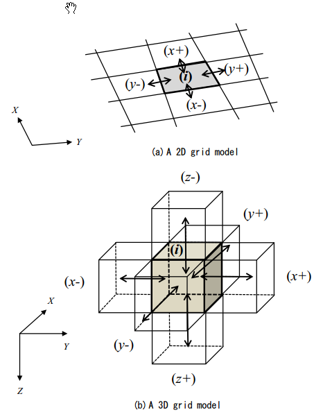
The Newton–Raphson method
The governing equations for the entire system, spatially discretized as shown in the previous section, formally describe the linear equation for an unknown variable X. However, the coefficient matrix is a function of unknown variables X, which has nonlinearity that depends on the state quantities of the field, which can vary from moment to moment. This nonlinearity is due to fluid properties included in the multi-phase flow model as functions of relative permeability, capillary pressure, pressure, and temperature; these are each treated as a function of saturation.
To obtain numerical solutions, GETFLOWS iterates (by the Newton–Raphson method) until convergence.
The nonlinear system of interest is described as a residual equation as follows.
\[\mathbf{R}\left( \mathbf{X} \right) = \mathbf{0}\qquad{(6.10)}\]
Iterative calculation by the Newton–Raphson method proceeds as follows.
(a) Set the initial value of \(\mathbf{X}^{0}\).
(b) Calculate the derivative \(\mathbf{R}\mathbf{'}\left( \mathbf{X}^{0} \right)\) of the function \(\mathbf{R}\left( \mathbf{X} \right)\) when \(\mathbf{X} = \mathbf{X}^{0}\). Calculation of the derivative function is by the following numerical differentiation method, using a small amount of change \(\mathbf{\Delta\text{X}}\) in the vicinity of \({\mathbf{X} = \mathbf{X}}^{0}\).
\[\mathbf{R}\mathbf{'}\left( \mathbf{X}^{0} \right)\mathbf{=}\frac{\mathbf{R}\left( \mathbf{X}^{0}\mathbf{+ \delta X} \right) - \mathbf{R}\left( \mathbf{X}^{0} \right)}{\mathbf{\Delta\text{X}}}\qquad{(6.11)}\]
The change \(\mathbf{\Delta\text{X}}\) comprises small changes in pressure and saturation, and sufficiently small values (for example, magnitudes of 10–8–10–10) are used for each, but these can be instead arbitrarily specified in the input data.
(c) Calculate \(\mathbf{R}\left( \mathbf{X}^{0} \right)\).
(d) Solve the following linear system to find a new trial value for \(\mathbf{X}^{1}\).
\[\mathbf{R}\mathbf{'}\left( \mathbf{X}^{0} \right)\left( \mathbf{X}^{1}\mathbf{-}\mathbf{X}^{0} \right) = - \mathbf{R}\left( \mathbf{X}^{0} \right)\] \[\mathbf{X}^{1}\mathbf{=}\mathbf{X}^{0}\mathbf{-}\frac{\mathbf{R}\left( \mathbf{X}^{0} \right)}{\mathbf{R}\mathbf{'}\left( \mathbf{X}^{0} \right)}\qquad{(6.12)}\]
(e) Repeat similar operations to derive \(\mathbf{X}^{v + 1}\).
\[\mathbf{R}\mathbf{'}\left( \mathbf{X}^{v} \right)\left( \mathbf{X}^{v + 1}\mathbf{-}\mathbf{X}^{v} \right) = - \mathbf{R}\left( \mathbf{X}^{v} \right)\qquad{(6.13)}\]
(f) Continue iterating until the following criterion is met.
\[\left| \mathbf{X}^{v + 1}\mathbf{-}\mathbf{X}^{v} \right| \leq \mathbf{\varepsilon}\qquad{(6.14)}\]
Here, \(\mathbf{\varepsilon}\) is a tolerance vector with components set to convergence thresholds. In practice, acceptable precision is obtained using magnitudes of 10–3–10–5 for pressure and saturation, and 10–7–10–9 for concentration.
Matrix solver
Linear equations for the overall discrete grid, created during the Newtonian iteration process, have asymmetric coefficient matrices (Jacobian matrices) with block sub-matrix components. Solutions to the matrix equations are obtained in GETFLOWS by the preconditioned conjugated residual method; this method combines a preprocessing method called nested factorization with the Orthomin method for processing large-scale asymmetric sparse matrices. An overview is provided below.
Nested factorization preprocessing
The asymmetric coefficient matrix of the linear equation takes the following form in a three-dimensional structured grid system:
\[\mathbf{A} = \mathbf{D} + \mathbf{L}\mathbf{1} + \mathbf{U}\mathbf{1} + \mathbf{L}\mathbf{2} + \mathbf{U}\mathbf{2} + \mathbf{L}\mathbf{3} + \mathbf{U}\mathbf{3} + N\qquad{(6.15)}\]
Here, \(\mathbf{A}\) is the asymmetric coefficient matrix, \(\mathbf{D}\) is the main diagonal, \(\mathbf{L}\mathbf{1}\), \(\mathbf{L}\mathbf{2}\), \(\mathbf{L}\mathbf{3}\) are the elements under the diagonal, and \(\mathbf{U}\mathbf{1}\), \(\mathbf{U}\mathbf{2}\), \(\mathbf{U}\mathbf{3}\) are the elements above the diagonal. N is a non-adjacent component, arising from cross-derivative components, linked faults, and other such things. Fig. 6.4 shows a 3D structured grid with \(NX = 4,\ NY = 3,\ NZ = 2\). Off-diagonal elements show interaction between grids, with \(\mathbf{L}\mathbf{1},\mathbf{U}\mathbf{1}\) being the interaction between adjacent innermost grid columns in a one-dimensional direction (one of x, y, z), \(\mathbf{L}\mathbf{2},\mathbf{U}\mathbf{2}\) the connection between grids for two grid columns in a second direction, and \(\mathbf{L}\mathbf{3},\mathbf{U}\mathbf{3}\) the interaction due to the connection between grids of two surfaces. As Fig. 6.5 shows, the structure of this coefficient matrix can be viewed as a nesting of tri-diagonal matrices, allowing application of the following incomplete Cholesky decomposition.
\[\mathbf{B} = \left( \mathbf{\alpha} + \mathbf{L3} \right)\mathbf{\alpha}^{- 1}\left( \mathbf{\alpha} + \mathbf{U}\mathbf{3} \right)\qquad{(6.16)}\] \[\mathbf{\alpha} = \left( \mathbf{\beta} + \mathbf{L}\mathbf{2} \right)\mathbf{\beta}^{- 1}\left( \mathbf{\beta} + \mathbf{U}\mathbf{2} \right)\qquad{(6.17)}\] \[\mathbf{\beta} = \left( \mathbf{\gamma} + \mathbf{L}\mathbf{1} \right)\mathbf{\gamma}^{- 1}\left( \mathbf{\gamma} + \mathbf{U}\mathbf{1} \right)\qquad{(6.18)}\]
Here,
\[\mathbf{\gamma}\mathbf{= D - L1}\mathbf{\gamma}^{\mathbf{- 1}}\mathbf{U}\mathbf{1 -}\text{colsum}\left( \mathbf{L2}\mathbf{\beta}^{\mathbf{- 1}}\mathbf{U}\mathbf{2 +}\mathbf{L3}\mathbf{\alpha}^{\mathbf{- 1}}\mathbf{U}\mathbf{3}\mathbf{+}\mathbf{N} \right)\mathbf{.}\qquad{(6.19)}\]
In this equation, \(\text{colsum}\mathbf{(}\mathbf{\varepsilon})\) is a diagonal matrix whose non-zero entries are the sums of the corresponding columns of the matrix \(\mathbf{\varepsilon}\). Matrix \(\mathbf{B}\) is a good approximation of the coefficient matrix \(\mathbf{A}\), allowing a numerical solution obtained by the Orthomin method, shown below, to finally calculate the nonlinear solution in each iterative step.

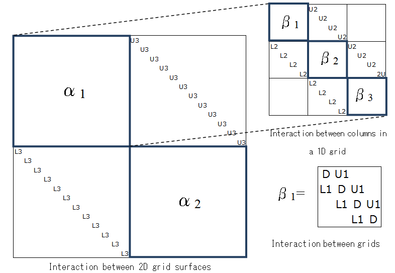
Iterative solutions using Orthomin
The Orthomin method is widely used as an iterative solver for simultaneous linear equations with large-scale sparse asymmetric coefficient matrices. The method mathematically guarantees monotonic decrease of the residual norm in determining the least squares solution and updates the approximate solution by using multiple iteratively obtained vectors.
For a linear system \(\mathbf{\text{AX}} = \mathbf{r}\) where \(\mathbf{A}\) is a coefficient matrix, the solution method using the approximate matrix \(\mathbf{B}\) described above is as follows.
(a) Obtain a new solution from the approximate matrix by using nested factorization.
\[\mathbf{p}^{\nu + 1} = \mathbf{B}^{- 1}\mathbf{r}^{\nu} = \left( \mathbf{\text{LU}} \right)^{- 1}\mathbf{r}^{\nu}\qquad{(6.20)}\]
(b) Use the following equation to obtain the orthogonal coefficient. The ratio of the numerator and denominator indicate the inner product of the vectors, and \(\mathbf{q}\) is the orthogonal vector.
\[a_{i}^{\nu + 1} = \frac{\left( \mathbf{\text{Aq}}^{i},\mathbf{\text{Ap}}^{v + 1} \right)}{\left( \mathbf{\text{Aq}}^{i},\mathbf{\text{Aq}}^{i} \right)},\ \ \ \ \ \ \ \ \ \left( i = 1,..,\nu \right)\qquad{(6.21)}\]
(c) Determine the following amount to minimize the least squares sum of the residual vector.
\[w^{\nu + 1} = \frac{\left( \mathbf{r}^{\text{v}\nu},\mathbf{\text{Aq}}^{\nu + 1} \right)}{\left( \mathbf{\text{Aq}}^{\nu + 1},\mathbf{\text{Aq}}^{\nu + 1} \right)}\qquad{(6.22)}\]
(d) Find the new orthogonal vector.
\[\mathbf{q}^{\nu + 1} = \mathbf{p}^{\nu + 1} - \sum_{i = 1}^{\nu}{\mathbf{a}_{i}^{\nu + 1}\mathbf{q}^{i}}\qquad{(6.23)}\]
(e) Find the new approximate solution and residual vector.
\[\mathbf{X}^{\nu + 1} = \mathbf{X}^{\nu} + w^{\nu + 1}\mathbf{q}^{\nu + 1}\qquad{(6.24)}\] \[\mathbf{r}^{\nu + 1} = \mathbf{r}^{\nu} - w^{\nu + 1}\mathbf{\text{Aq}}^{\nu + 1}\qquad{(6.25)}\]
(f) Perform a convergence test using the Euclidean norm of the residual vector. Here, \(\mathbf{r}^{0}\) is the initial norm of the residual vector. Repeat the process described above until the convergence criteria are met.
\[\|\mathbf{r}^{\mathbf{\nu}} + 1\|/\|\mathbf{r}^{0}\ \|\ \leq \mathbf{\varepsilon}\qquad{(6.26)}\]
Convergence conditions for the matrix solution
GETFLOWS generally uses either relative residuals (current residual sum of squares / initial residual sum of squares) or absolute residuals (current sum of squares of the residual) as the residual sum of squares convergence condition. In most cases, an extremely small value (approximately \(\varepsilon = {1.0e}^{- 10}\)) is used for absolute residual determination, which provides solutions with sufficiently high accuracy. Increasing accuracy to this extent requires from several up to twenty iterations. In most cases, the rate of convergence in Newton’s method is increased with better precision of the ranks solution.
Acceleration and Stabilization Options
Successive Locking Process
GETFLOWS contains an option for implementation of a successive locking process (SLP), by which state changes to factors such as pressure and saturation are monitored in each grid during nonlinear calculation iterations, and grids exhibiting sufficiently small change are successively excluded from the solver, which reduces the calculation load. The determination as to whether change in a grid is sufficiently small is made by reference to input threshold values (the SLP conditions), as expressed in the following inequality.
\[\left| \begin{matrix} \delta\mathbf{x}_{i - 1}^{n} \\ \end{matrix} \right|^{v} \leqq \mathbf{\varepsilon}^{n}\text{\ \ \ }\left( n = 1,..,M \right)\qquad{(6.27)}\]
Here, \(\delta\mathbf{x}_{i - 1}^{n}\) is the state quantity for a fluid phase n in grid \(i - 1\), indicating various quantities in the vth iteration. The value of \(\mathbf{\varepsilon}^{n}\) is a small value used to determine the amount of state variation of each grid, and is a component of the input threshold value. M is the number of equations for each grid, which varies according to the fluid system of interest. In the case of a water–air two-phase system, where water and air are of interest, \(M = 2\).
The numerical solution of a grid \(i - 1\) satisfying the SLP condition is locked by the following equation.
\[\mathbf{X}_{i - 1}^{(L + 1)} = \mathbf{X}_{i - 1}^{(L)} + \sum_{v = 1}^{v}{\delta\mathbf{X}}_{i - 1}^{v}\qquad{(6.28)}\]
Here, \(L,\ L + 1\) are simulation steps. The state quantities (pressure, saturation) of grids excluded because they met the SLP condition in the iterative nonlinear calculation process are locked, with between-grid flows preserved in the following steps.
Fig. 6.6 shows the concept of flow between grids and adjacent grids meeting the SLP conditions. Between a grid \(i - 1\) fulfilling the SLP conditions and left–right adjacent grids \(i - 1\) and \(i\), in the nonlinear iterative calculation that follows, flow rates Qi,x and Qi-2,x+ are each preserved as follows.
\[{Q_{f}}_{i,x -}^{m,(L + 1)} = {Q_{f}}_{i,x -}^{m,(v)}\text{\ \ \ \ \ }\ \ (m = 1,2,\ldots M)\qquad{(6.29)}\] \[{Q_{f}}_{i - 1,x +}^{m,(L + 1)} = {Q_{f}}_{i - 1,x +}^{m,(v)}\text{\ \ \ \ \ }\ \ (m = 1,2,\ldots M)\]
Here, \({Q_{f}}_{i,x -}^{m,(v)}\) is the flow amount of fluid phase m passing through the left side (the X– face) of grid i in the vth iteration. This flow is locked in successive nonlinear iterative calculations, and used as flow \({Q_{f}}_{i,x -}^{m,(L + 1)}\) in the next timestep \(L + 1\). Similarly, \({Q_{f}}_{i - 1,x +}^{m,(v)}\) is the flow amount of fluid phase m passing through the right side (the X+ face) of grid \(i - 1\) in the vth iteration, and this flow is used as flow \({Q_{f}}_{i - 1,x +}^{m,(L + 1)}\) in the next step.
Such processing means that flow variation between a grid satisfying the SLP conditions and adjacent grids is ignored during the remaining nonlinear iterative calculations. This approximation has been confirmed as being reasonable for the numerical solution of partial differential equations in ranges for which sufficiently small threshold values have been supplied to determine whether the SLP conditions are met.
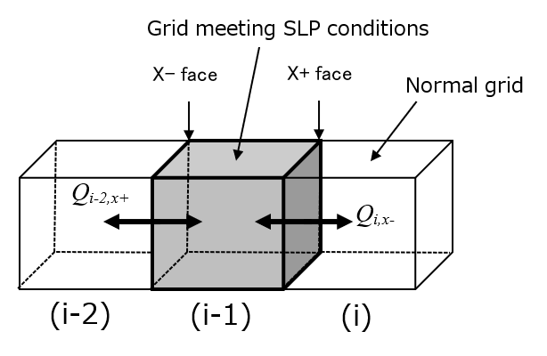
Automatic Time Step
GETFLOWS allows for two methods for setting the timestep \(t\) used in calculations: a method that uses a previously set fixed timestep, and one that automatically determines the timestep.
When a fixed timestep is used, a combination of the timestep \(t\) and the number of steps during which it should be used are directly indicated. In the method for automatically determining the timestep, differences resulting from increased timesteps in the simulation allows further selection between the following two methods.
Method A
Determination of convergence on a numerical solution during the solution-finding process is performed in the linear solver by the conjugate residual method and the nonlinear iterative process of the Newton–Raphson method, with the determination standards of each as previously described.
When neither of these methods fulfills the convergence condition, GETFLOWS resets the timestep and repeats the solution-finding process with the new value. When the convergence condition is met, the supplied coefficient is used to increase the next step, and the simulation proceeds to the solution-finding process for the next timestep as itemized here.
(a) Timestep \(t^{n}\) is used to obtain a numerical solution for simulation step \(n\).
(b) If the method converges, update the timestep by the following equation, where C is larger than 1.
\[{t}^{n + 1} = C \bullet {t}^{n}\qquad{(6.30)}\]
(c) Proceed to the next simulation step and use the new timestep \({t}^{n + 1}\) for that step.
(d) Otherwise, update the timestep by the following equation.
\[{t}^{n} = {t}^{n}/2\qquad{(6.31)}\]
(e) Try the new timestep \({t}^{n}\) to obtain a numerical solution for simulation step \(n\).
(f) Repeat steps (a) through (e) above for all simulation steps.
In the above method, the accuracy of the numerical solutions and calculation efficiency will vary with the provided coefficient C. Larger values will allow long-term simulations with fewer calculation steps but will also increase the amount of change, resulting in more non-convergence, which will entail repeated trial calculations. In contrast, smaller values of C will reduce the number of repeated trial calculations, but the number of calculation steps required for simulating a given simulation step will increase. Determining the most appropriate coefficient for a given situation will likely require trying different values in conditioning calculations to best adjust to the characteristics of each analysis. Typically, values between 1.1 and 1.2 are used.
Method B
This method sets timesteps such that the state quantity change between adjacent grids does not exceed a predefined limit value. In the case of a water–air two-phase system, the state quantities used are saturation and pressure .
(a) Find the maximum values for saturation and pressure change between adjacent grids at simulation step n by using the following.
\[\left( \text{DS} \right)_{\max}^{n} = \max_{\text{ijk}}\left\{ {_{t}S_{\text{ijk}}}^{n} \right\}\qquad{(6.32)}\] \[\left( \text{DP} \right)_{\max}^{n} = \max_{\text{ijk}}\left\{ {_{t}P_{\text{ijk}}}^{n} \right\}\qquad{(6.33)}\]
Here, \({_{t}S_{\text{ijk}}}^{n}\) and \({_{t}P_{\text{ijk}}}^{n}\) are, respectively, the amounts of saturation and pressure change occurring between adjacent grids in three dimensions, and these determine the maximum amount of change.
(b) Use the following equation to find a new timestep \({t}^{n + 1}\) for simulation step \(n + 1\).
\[{t}^{n + 1} = min\left\{ {t}_{s},{t}_{p} \right\}\qquad{(6.34)}\]
Here, \({t}_{s},{t}_{p}\) are the timesteps calculated from the maximum change in saturation and pressure at simulation step n, according to the following equation.
\[{t}_{s} = {t}^{n}\frac{\text{DS}_{\text{limt}}}{\left( \text{DS} \right)_{\max}^{n}},\ \ {t}_{p} = {t}^{n}\frac{\text{DP}_{\text{limt}}}{\left( \text{DP} \right)_{\max}^{n}}\qquad{(6.35)}\]
Here, \(\text{DS}_{\text{limt}},\text{DP}_{\text{limt}}\) are input values specifying the limits for quantity change in saturation and pressure, which will vary with the problem. The value of \(\text{DS}_{\text{limt}}\) is typically in the range 0.05–0.10. This method sets timesteps such that the respective quantities of change for saturation and pressure reach the limits \(\text{DS}_{\text{limt}},\text{DP}_{\text{limt}}\), but the timestep has a nonlinear relation with quantities of change for saturation and pressure, so timesteps sometimes allow exceeding this range.
(c) After performing analysis for simulation step \(n + 1\), the following process is performed so that the specified limits on maximum quantity of change are not exceeded.
\[\left( \text{DS} \right)_{\max}^{n + 1} \leq C_{1} \times \text{DS}_{\text{limt}},\ \ \left( \text{DP} \right)_{\max}^{n + 1} \leq C_{2} \times \text{DP}_{\text{limt}}\qquad{(6.36)}\]
Here, \(C_{1},\ C_{2}\) are coefficients greater than 1. A new timestep is calculated using these by the following equation.
\[{t}^{*} = min\left\{ {t}_{s},{t}_{p} \right\}\qquad{(6.37)}\]
Here,
\[{t}_{s} = {t}^{n + 1}\frac{\text{DS}_{\text{limt}}}{\left( \text{DS} \right)_{\max}^{n + 1}},\ \ {t}_{p} = {t}^{n + 1}\frac{\text{DP}_{\text{limt}}}{\left( \text{DP} \right)_{\max}^{n + 1}}\qquad{(6.38)}\]
(d) Simulation step \(n + 1\) is recalculated with \(\ {t}^{n + 1}\) set to \({t}^{*}\).
(e) The above steps (a) through (d) are repeated for each simulation step.
Damped Newton Iteration
In the nonlinear iterative process by Newton’s method, if no solution is converged upon (there is no convergence within the specified number of iterations as a result of non-diverging oscillation), this can cause activation of the automatic timestep determination process, which can result in extremely small timestep values. Solution damping avoids such situations by allowing calculations with large timesteps when near convergence is obtained.
In the Newton iterative process, the maximum absolute value of a feasible solution becomes gradually smaller, and when convergence is achieved to within \(\gamma\) times the convergence threshold, the solution vectors passed by the matrix solver are added to the current value as a multiple of \(\alpha\ (\alpha = 0.5)\). This operation suppresses overshooting the solution near the convergence limit, allowing a smoother approach toward the solution. There are many cases where setting an appropriate value for \(\gamma\) and proceeding with large timesteps under this option allows a significant decrease in calculation time.
Parallel Processing – Domain Decomposition Methods
GETFLOWS allows division of the full analysis region into multiple partial regions, enabling domain decomposition in which the analysis of results for border regions are exchanged to allow for region-specific solutions . Applying this method of domain decomposition can be effective in situations where there are extreme imbalances in the state change of pressure and saturation, or when parallel processing is to be performed.
Fig. 6.7 shows this concept applied to an analysis area decomposed into four partial regions, D1–D4. Thick lines in the figure indicate partial region borders, and adjacent grids touching along this border share pressure and saturation state quantities, with fluid transfer allowed between them. Dividing the full area into partial regions in this manner can in some cases lower the accuracy of numerical solutions because of splitting errors caused by the inter-regional data exchange. In such cases, bordering partial regions should be supplied with a shared transitional region. The dashed lines in the figure indicate the boundaries of such a shared transitional region along the partial region borders. Arbitrary values can be specified for the grid range forming this transitional region, as appropriate to the problem of interest.
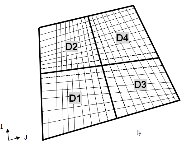
Mathematically speaking, this can be described as a time evolution of the state quantity change at time t of each partial region, as follows.
\[\begin{Bmatrix} \begin{matrix} {\dot{\mathbf{x}}}_{1} \\ {\dot{\mathbf{x}}}_{2} \\ \end{matrix} \\ \begin{matrix} {\dot{\mathbf{x}}}_{3} \\ {\dot{\mathbf{x}}}_{4} \\ \end{matrix} \\ \end{Bmatrix}_{t} = \begin{bmatrix} \begin{matrix} \mathbf{A}_{11} & \mathbf{A}_{12} \\ \mathbf{A}_{21} & \mathbf{A}_{22} \\ \end{matrix} & \begin{matrix} \mathbf{A}_{13} & \mathbf{A}_{14} \\ \mathbf{A}_{23} & \mathbf{A}_{24} \\ \end{matrix} \\ \begin{matrix} \mathbf{A}_{31} & \mathbf{A}_{32} \\ \mathbf{A}_{41} & \mathbf{A}_{42} \\ \end{matrix} & \begin{matrix} \mathbf{A}_{33} & \mathbf{A}_{34} \\ \mathbf{A}_{43} & \mathbf{A}_{44} \\ \end{matrix} \\ \end{bmatrix}_{t}\begin{Bmatrix} \begin{matrix} \mathbf{x}_{1} \\ \mathbf{x}_{2} \\ \end{matrix} \\ \begin{matrix} \mathbf{x}_{3} \\ \mathbf{x}_{\mathbf{4}} \\ \end{matrix} \\ \end{Bmatrix}_{t} + \begin{Bmatrix} \begin{matrix} \mathbf{q}_{1} \\ \mathbf{q}_{2} \\ \end{matrix} \\ \begin{matrix} \mathbf{q}_{3} \\ \mathbf{q}_{4} \\ \end{matrix} \\ \end{Bmatrix}\qquad{(6.39)}\]
Here, \(\mathbf{x}_{i}\) is a state quantity vector comprising grid pressure, saturation, concentration, temperature, and other states for partial region \(i\ (i = 1,2,3,4)\), and \({\dot{\mathbf{x}}}_{i}\) is the change over time. In the first term on the right, \(\mathbf{A}_{\mathbf{i},j}\mathbf{(}i \neq j)\) is a coefficient matrix representing interaction between partial regions i and j \((j = 1,2,3,4)\), and the \(i = j\) values form the coefficient matrix for the partial region itself. The vector \(\mathbf{q}_{i}\) is the external force vector corresponding to the production and injectivity terms.
The above equation can use the state quantity of the immediately preceding simulation step as the state quantity of an adjacent partial region for the following approximation.
\[\begin{Bmatrix} \begin{matrix} {\dot{\mathbf{x}}}_{1} \\ {\dot{\mathbf{x}}}_{2} \\ \end{matrix} \\ \begin{matrix} {\dot{\mathbf{x}}}_{3} \\ {\dot{\mathbf{x}}}_{4} \\ \end{matrix} \\ \end{Bmatrix}_{t} \cong \left\lbrack \begin{matrix} \text{\ \ }\mathbf{A}_{11}\mathbf{\text{\ \ }} \\ 0 \\ 0 \\ 0 \\ \end{matrix}\begin{matrix} 0 \\ \mathbf{A}_{22}\mathbf{\text{\ \ }} \\ 0 \\ 0 \\ \end{matrix}\begin{matrix} 0 \\ 0 \\ \mathbf{A}_{33}\mathbf{\text{\ \ }} \\ 0 \\ \end{matrix}\begin{matrix} 0 \\ 0 \\ 0 \\ \mathbf{A}_{44}\mathbf{\text{\ \ }} \\ \end{matrix} \right\rbrack_{t}\begin{Bmatrix} \begin{matrix} \mathbf{x}_{1} \\ \mathbf{x}_{2} \\ \end{matrix} \\ \begin{matrix} \mathbf{x}_{3} \\ \mathbf{x}_{\mathbf{4}} \\ \end{matrix} \\ \end{Bmatrix}_{t} + \boxed{\begin{Bmatrix} \begin{matrix} {\mathbf{A}_{\mathbf{12}}\mathbf{x}}_{\mathbf{2}}\mathbf{+}{\mathbf{A}_{\mathbf{13}}\mathbf{x}}_{\mathbf{3}}\mathbf{+}{\mathbf{A}_{\mathbf{14}}\mathbf{x}}_{\mathbf{4}} \\ \mathbf{A}_{\mathbf{21}}\mathbf{x}_{\mathbf{1}}\mathbf{+}\mathbf{A}_{\mathbf{23}}\mathbf{x}_{\mathbf{3}}\mathbf{+}\mathbf{A}_{\mathbf{24}}\mathbf{x}_{\mathbf{4}} \\ \end{matrix} \\ \begin{matrix} \mathbf{A}_{\mathbf{31}}\mathbf{x}_{\mathbf{1}}\mathbf{+}\mathbf{A}_{\mathbf{32}}\mathbf{x}_{\mathbf{2}}\mathbf{+}\mathbf{A}_{\mathbf{34}}\mathbf{x}_{\mathbf{4}} \\ \mathbf{A}_{\mathbf{41}}\mathbf{x}_{\mathbf{1}}\mathbf{+}\mathbf{A}_{\mathbf{42}}\mathbf{x}_{\mathbf{2}}\mathbf{+}\mathbf{A}_{\mathbf{43}}\mathbf{x}_{\mathbf{3}} \\ \end{matrix} \\ \end{Bmatrix}_{t - t}} + \begin{Bmatrix} \begin{matrix} \mathbf{q}_{\mathbf{1}} \\ \mathbf{q}_{\mathbf{2}} \\ \end{matrix} \\ \begin{matrix} \mathbf{q}_{\mathbf{3}} \\ \mathbf{q}_{\mathbf{4}} \\ \end{matrix} \\ \end{Bmatrix}\qquad{(6.40)}\]
The first term on the right is the state change term for the diagonalized (non-coupled) partial region, and the second term is the interaction term for the area between adjacent partial regions. This interaction term is approximated by the state quantity previously calculated at the beginning of the prior simulation step, and can be used as the external force term for the partial region.
The second term on the right is the interaction term between partial regions.
Division of regions will necessarily cause splitting errors through the interaction term, which is evaluated by using the state quantity from the immediately preceding simulation step. The extent of such splitting errors depends on factors such as the nature of the problem, the method used to divide the region, and differences in the shared transitional region. In practice, several trial calculations should be performed to obtain a general understanding of the influence that domain division has on the accuracy of numerical solutions in the specific case.
Note that in cases where parallel processing will be performed on multiple CPUs, different processors will be awaiting calculation processing of each partial region, and the interaction term for adjacent partial regions is obtained and calculated using only the data needed for each processor. In cases where there are large differences in the computational load between regions, the method of division or method for processor allocation should be altered.
Program Flow
With the exception of some libraries, most of the I/O processing and solver units in GETFLOWS were written in FORTRAN 90/95. Fig. 6.9 shows the processing flow of major components of the main program. The program is roughly composed of input and initialization, iterative calculation processing, and output processing units.
The input and initialization unit reads input data, sets up the number of phases and number of components for the fluid system of interest, and creates the 3D grid model. Physical properties of each fluid phase, such as concentration and viscosity coefficients, are initialized according to the initial state quantities for pressure, saturation, and similar properties. The 3D grid model is constructed on the basis of corner-point coordinates read in from the input data, starting with a check for the presence of obviously erroneous input (e.g., duplicated coordinate values and ordering violations). If erroneous corner-point coordinates are found, then the program outputs an error message and information regarding the problematic grid, following which it terminates. If no erroneous corner-point coordinates are found, then the program calculates geometric data, such as the volume of each grid, center of gravity coordinates, and the surface area between adjacent grids, and applies geologic strata properties, such as permeability and effective porosity, to each grid. Finally, an array of principal variables, such as pressure and saturation, is initialized, and iterative calculation processing begins.
The iterative calculation processing unit identifies the standard RUN mode or OBS mode for operation. In RUN mode, standard iterative calculation is performed according to the provided input data. In OBS mode, a previously calculated result’s data are used for output processing of flow volume, water level, and the like.
In OBS mode, main output data previously calculated during the simulation loop are read sequentially, all iterative solver calculations are skipped, and only the output data are provided. The main GETFLOWS output data consist of principal variables related to pressure, saturation, temperature, and concentration for each grid cell, stored in a binary format. Between-grid flow and water level are provided as secondary variables that can be calculated from the principal variables. OBS mode is used for follow-up output of principal variables and the recalculation of secondary variables.
The normal RUN mode reads and updates external force conditions sequentially at each calculation step of the time loop. External force conditions depend on factors such as rainfall, evaporation, and the heat source for thermal elements. In the nonlinear loop, Jacobian matrices and residual vectors are constructed while sweeping through directional components, and the Newton–Raphson method is applied to iteratively converge on numerical solutions. Conditions for determination of convergence are supplied as the maximum change value for principal variables such as pressure and saturation in each grid, the timestep is adjusted such that convergence occurs within the input tolerance range, and calculations are repeated.
Note that in cases where successive locking is used, as described below, differential grids with small change quantities in the nonlinear iterative calculation process are dynamically excluded from the solver.
In the output processing unit, principal variables (pressure, saturation, concentration, temperature) related to all differential grids are output for each step, as specified by the input. This main output file often becomes quite large, and so is written in a binary format. Time series data for variables at a specific point, such as between-grid flow, concentration, and water level, can be output at each input-specified step in ASCII format to an arbitrary storage device.
The method for constructing Jacobian matrices and residual vectors varies with the fluid system of interest, roughly divided into isothermal fluid systems, non-isothermal fluid systems, and multi-component mass transport. Fig. 6.9 shows the main steps in the processing flow for matrix construction for a multi-phase multi-component system under isothermal conditions.
First, in each nonlinear calculation iteration for a given simulation step, fluid properties are calculated and updated according to state quantities such as pressure and saturation. These values are used to evaluate each component of the Jacobian matrix. Next, after initializing the Jacobian matrix and array of residual vectors, the terms forming the mass conservation equation for each fluid phase and material component are evaluated.
For water, air, and NAPL fluid phases, the flow and retention terms for each are first evaluated. Jacobian matrix elements are divided among multiple arrays and stored, with diagonal terms stored in the 1-column DIAG(N) array, and above-diagonal and below-diagonal terms stored, respectively, in the SUPD(N,3) and SUBD(N,3) 2-column arrays. Residual vectors are stored in the 12-column RESD(N) array. Here, N is the number of rows, which will vary with the number of grids in the fluid system of interest, with \(N=NEQ^{2} \times NNBLK \times NEQ\) and NNBLK are respectively the number of principal variables in each grid (in other words, the number of mass balance equations) and the number of grids. Arrays of above- and below-diagonal terms store three-dimensional direction components, so three times the number of diagonal components are reserved.
When material transport in water (liquid) or air (gaseous) phases is considered, mass conservation equations are created for each material component of interest, so terms for advection, diffusion/dispersion, adsorption, and decomposition/decay are evaluated. When interphase material transport—such as NAPL dissolution into liquid phases, NAPL volatilization into gaseous phases, or gaseous dissolution into liquid phases—is considered, interphase transport terms are evaluated, and the Jacobian matrix and residual vectors are updated accordingly.
After mass conservation equations have been constructed for all fluid phases and material components, production and injectivity terms, rainfall terms, and evapotranspiration terms are evaluated, and the Jacobian matrix and residual vectors are updated accordingly.
For non-isothermal fluid systems, energy conservation equations describing heat transport in fluids and geologic media are added and reflected in the Jacobian matrix and residual vectors (Fig. 6.10). Specifically, these conservation equations are terms for head advection and conduction in a gas–liquid mixture fluid and in soil or solid rock phases. Heat exchange terms between fluid and solid phases are also added. Mass conservation equations for water vapor are constructed in the materials loop, and terms for advection, diffusion/dispersion, adsorption, and production/dissolution (including water vapor generation/condensation) are evaluated.
Each of the above evaluations are used for fluid properties as they change over time with the temperature field.
Fig. 6.11 shows the processing flow for multi-component material transport calculations. Processing assumes a solution system with dilute concentration, and the velocity field is used as a previously calculated condition for evaluation of the advection term. The velocity field is sequentially read from a previously calculated input file, and recalculated as a between-grid flow rate for each direction at each simulation step. In cases where the assumption of a dilute solution system does not hold, the mutual interference between the concentration and velocity fields are considered according to the process shown in Fig. 6.9.


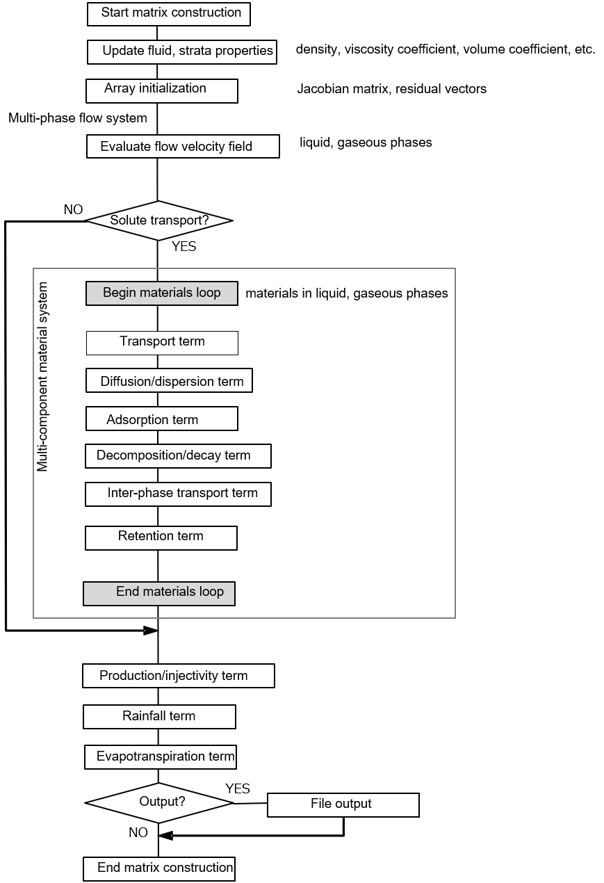
References
©General-purpose Terrestrial Fluid Flow Simulator User’s Manual - All Rights reserved
| First version: 18 Aug 2010 |
| Geosphere Environmental Technology Corp., Chiyoda Ward, Tokyo |
| https://www.getc.co.jp |
@Copyright Geoshpere environmental technology Corp. All Rights reserved.
A fluid having affinity with a solid phase is called a wetting phase fluid. Water is generally a wetting–phase fluid for soil and rock, so under non-saturated conditions capillary effects will result in water being pulled (absorbed) into pores. When there is a mixture of water and oils, the water portion is generally the wetting phase, and the oil portion is the non-wetting phase (the reverse case is also possible, such as with oil rock). In the case where air coexists with a liquid, it is always a non-wetting phase fluid and is discharged through suction by a wetting phase fluid (source: Groundwater Science Glossary of the Japanese Association of Groundwater Hydrology).↩︎
A fluid having affinity with a solid phase is called a wetting phase fluid. Water is generally a wetting–phase fluid for soil and rock, so under non-saturated conditions capillary effects will result in water being pulled (absorbed) into pores. When there is a mixture of water and oils, the water portion is generally the wetting phase, and the oil portion is the non-wetting phase (the reverse case is also possible, such as with oil rock). In the case where air coexists with a liquid, it is always a non-wetting phase fluid and is discharged through suction by a wetting phase fluid (source: Groundwater Science Glossary of the Japanese Association of Groundwater Hydrology).↩︎