Card input file system - user manual
Geosphere Environmental Technology Corp.
v0-11-0 – 2021/07/01
Introduction
Card Input is an input file system for GETFLOWS that
can be used as a replacement of the standard base Input
system (job-pvt-blk). Under the hood, the card input
file system is converted to a base Input file system used
by GETFLOWS to set up a computation job and run a simulation. The syntax
is currently at its second version.
Compare to the base Input file system, the card input file system is flexible, self-documented, and contains several defaults value that help the first steps with the simulator. The key features of the card input file system are as follow.
It is possible to set up all the parameters in one unique file. Reference to external files from the main input file is also possible.
Thanks to the unified syntax, all parameters are set up in the same structured, self-documented syntax.
Default values are defined for several parameters including the linear solver parameters and the time step control parameters. This feature significantly reduces the minimal number of required user input.
Reusable sets of parameters (for solid and fluid properties) can be defined in objects.
Despite their difference, Card Input and Base Input file systems also shares several points. For the sake of completeness, they are presented in this manual. Knowledge of the Base Input file system is not mandatory to follow this manual.
Usage
How to run GETFLOWS
Running GETFLOWS with the card-input file-system requires to process
the card-input files and to execute GETFLOWS program. The preprocessor
program is called cardprocess while the simulator program
is simply called GETFLOWS. The steps are as follow:
- Run
cardprocesswith the suitable arguments - Run
GETFLOWSexecutable file
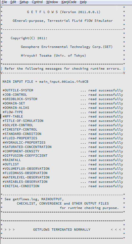
The status of the loaded dataset and the output information are displayed on the standard output (console) as well as in some log files.
It is possible to run GETFLOWS with the card-input file system using
one commmand. The command name is cardrun. Typing
cardrun input.gfcard in a terminal will execute both the
preprocessor and the simulator
 {#fig:GETFLOWSRuntime
height:600px}
{#fig:GETFLOWSRuntime
height:600px}
Job files
Job input file
A simulation case is called a calculation job or a job. Each job defines an independent case with its associated input and output files as shown on Fig. 2.1. When GETFLOWS is executed, the Card Input input files are loaded and the base Input files are prepared by the pre-processor. Then, the computation starts and the necessary output files are created. During the computation process, GETFLOWS continues to access to the output file, so these files should not be edited or deleted until the simulation finish. While names of input and output files are arbitrary, it is usually a good practice to conform to the naming convention used in this manual.
Note that GETFLOWS is available for the operating systems Linux and Windows.

File system
Input file system
The card input files system consists the job file and the (optional) external files (Table 2.1).
The job file contains the necessary input data for the simulator execution, directly into the file or via links to external files. External files are useful to input large set of data like the grid file or the hot restart file. Data that are seldomly modified can also benefit being put in external files. Moreover, the external files can be stored in binary format to shorten the loading time and reduce the disk space requirement. Any file name can be chosen for the main input file and the external input files.
Output file system
GETFLOWS computation results are stored into several output files that are set up in the job file. Table 2.2 lists the output files generated by GETFLOWS. Among them, the main output file, the convergence monitoring files and the primary variables file are the most important ones.
The information on the input configuration is summarized in the main
output file. The primary variables file contains the primary variables
computed at all grid cells in a binary format. Binary file format is
used for potentially large file to increased data capacity and ease
frequent restart. The monitoring convergence files store in the
iterative process some relevant parameters from the linear and nonlinear
solvers, such as the number of iterations, the maximum variation of
primary variables during two iterations, the volume status, or the norm
of the computed errors. These Base output files are created when
GETFLOWS is in RUN mode, which means that the input
parameters are loaded and the computation is running.
Other output files are generated in the RUN mode but
also in the POST mode where only output files are created
from existing computation results. The name of each file is arbitrary.
Some large files such as the restart file or the interstitial velocity
are usually written in binary format.
| File | Name | Type | Contents |
|---|---|---|---|
| Main input file | Any | ASCII | Contains the input parameters of a given simulation scenario. |
| External input files | Any | ASCII or BINARY | Contains additional input data that are not directly input in the main input file. The main input file should contains the paths to the external files. External input files are often used to store large dataset or data that don’t change between simulation scenarios. If all the necessary input data are directly define in the main input file, using external input file is not necessary. |
| # | File type | Name | Type | Contents |
|---|---|---|---|---|
| 1 | Main output | Any | ASCII | Loaded input information, error messages, main results |
| 2 | Primary variables | Any [main.bin] | BINARY | Primary variables computed on all grid cells (binary format used for visualization and restart) |
| 3 | Convergence monitoring | Any [solver.dat] | ASCII | Some relevant parameters at each iteration |
| 4 | Rain | Any [rain.xxx] | ASCII | Historical precipitation data |
| 5 | Well | Any [well.xxx] | ASCII | Well historical data (bottom hole pressure, flow, etc.) |
| 6 | Well group | Any | ASCII | Well historical data (bottom hole pressure, flow, etc.) |
| 7 | Evapo-transpiration | Any | ASCII | Historical evapotranspiration data |
| 8 | Evapo-transpiration | Any | BINARY | Same as above (only binary file for restart) |
| 9 | Sea-level change | Any | ASCII | Sea-level change history data |
| 10 | Change properties | Any [volumeFlux] | ASCII | Properties change history data |
| 11 | Checklist | Any | ASCII | User specified output data |
| 12 | Fluid mass | Any | ASCII | Fluid mass of the designated grid cells |
| 13 | Primary variables | Any | ASCII | Primary variables of the designated grid cells |
| 14 | Interstitial flow | Any | ASCII | Flow rate through a designated cross-section cells |
| 15 | Interstitial flow rate | Any | BINARY | Interstitial flux in all grid cells |
| 16 | Water level | Any | ASCII | Water level elevation value of the designated grid cells |
GETFLOWS system
Units system
The units system for the physical parameters is listed below. Note that for some input data such as rainfall and evapotranspiration, the user can specify its own unit.
| Physical parameter | Unit | Unit (full text) |
|---|---|---|
| Acceleration of gravity | m/s2 | meter per second squared |
| Corner point coordinates | m | meter |
| Time | day | day |
| Pressure | kgf/cm2 | kilogram-weight per square centimeter |
| Saturation factor | - | dimensionless |
| Viscosity coefficient | cP | centipoise |
| Density | g/cm3 | gram per cubic centimeter |
| Equivalent roughness coefficient | m-1/3s | |
| Effective porosity | - | dimensionless |
| Absolute permeability | mD | millidarcy |
| Relative permeability | - | dimensionless |
| Aqueous level | m | meter |
| Mass | kg | kilogram |
| Volume | m3 | cubic meter |
| Flow | m3/d | cubic meter per day |
Grid system
Coordinates
GETFLOWS is based on a Cartesian coordinate system. The origin of vertical axis (Z axis) corresponds to zero meter elevation relative to sea level, and the direction of increasing coordinates is oriented toward the opposite of the elevation.
Cells numbering
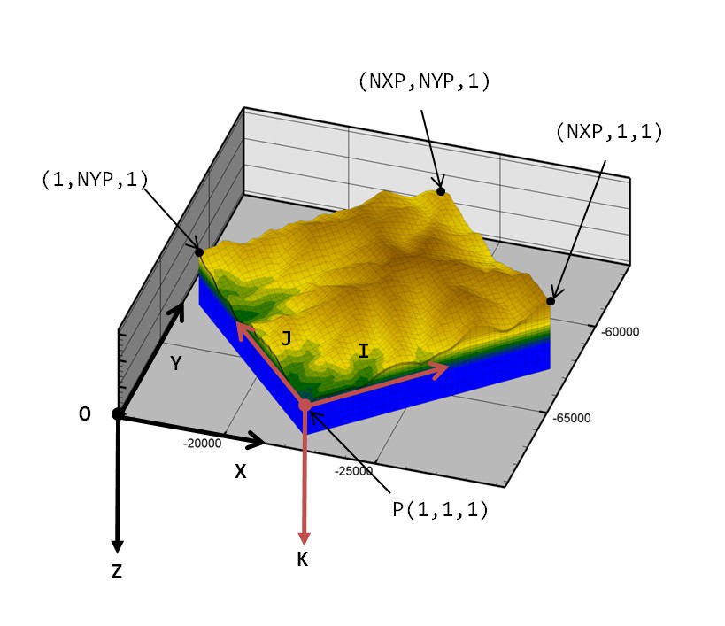
Fig. 3.1 shows the three-dimensional Cartesian coordinate system and the cell numbering convention of GETFLOWS. As mentioned earlier, in GETFLOWS, the Z-axis direction is oriented toward the decreasing elevation. In the figure, O-XYZ is the Cartesian coordinate system and the IJK P-coordinate system attached to the corner of the cell designs the cell numbering convention.
The I-axis direction is oriented toward the increasing coordinate value X, the J-axis is defined as the direction of increasing coordinate value Y and the K-axis is defined as the direction of increasing coordinate value Z. Note that the axis of the IJK coordinate system are not necessary parallel to the axis of the XYZ Cartesian coordinate system. Moreover, the O-IJ 2D system does not have to be orthogonal. The origin of the IJK P-coordinate system is defined in one corner of the model, as shown in Fig. 3.1. The relationship between the total number of cells in each direction (NX, NY and NZ) and the corresponding maximum coordinate (NXP, NYP and NZP) is given by:
NXP = NX + 1
NYP = NY + 1
NZP = NZ + 1
If no Local Grid Refinement (LGR) is defined, the total number of grid cells (NNBLK) and the total number of coordinates (NNBLKP) are given by:
NNBLK = NX \* NY \* NX ! Total number of grid cells
NNBLKP = NXP \* NYP \* NZP ! Total number of coordinates
When designing an arbitrary grid cell, the cell number is assigned by dividing each IJK axis. This is commonly used in the creation of input-output data. GETFLOWS assigns a number to each cell sequentially following this rule: the cell number 1 is the cell with the coordinates (1,1,1). Then, the cell number increase with the increasing I followed by the increasing J after I=NX and finally increasing K after J=NY. This leads to the following formula to express the cell number NB with the coordinates IJK:
NB = I + (J - 1) \* NX + (K - 1) \* NX \* NYThe resulting sequence of numbers is used to store the computed primary variables.
Cell attributes
Each cell defined in the previous section is a hexahedral cell with eight vertices (or corner points). The coordinates of each vertex are arbitrary; therefore it is possible to model complex spatial shapes, such as topography and strata. Fig. 3.2 shows the cell numbered (I, J, K) with a schematic diagram. The corner point number (I1, J1, K1) is shown in the figure.
Some physical properties such as the effective porosity and the
absolute permeability are assigned to each cell. These attributes are
divided into those assigned on the side of the cell and those assigned
on the entire cell. To be able to give an attribute to a given side of a
cell, each cell side is designed with an identifier: the letter of the
direction (I, J or K) followed by - if the side tangent
output vector is oriented toward the decreasing values or +
if the tangent vector is oriented toward the increasing values. The cell
side designation is also used when one needs to specify the flow through
a given side or when considering the anisotropy of the medium.

Type of simulation
Different types of simulation are implemented based on the water-gas two-phase flow analysis. In Table 3.2, the analysis type and their corresponding properties are listed (for instance, NAPL, heat, and chemical species). The simulation type should be chosen depending on the project requirements. Note that the number of equations per grid cell (NEQ), the number of phases (NPH) and the fluid systems depend on the simulation.
| Number of equations (NEQ) | Number of phase (NPH) | Aqueous | Gas | NAPL | Chemical species (NC) | Heat | Swimming sand Bed load | |
|---|---|---|---|---|---|---|---|---|
| Water-gas two-phase flow analysis | 2 | 2 | ✓ | ✓ | ✓ | |||
| Density flow analysis | 3 | 2 | ✓ | ✓ | ✓ | |||
| Water-gas-NAPL three-phase flow analysis | 5 | 3 | ✓ | ✓ | ✓ | ✓ | ||
| Reactive mass transport analysis (cf. note) | NC | 2 | (✓) | (✓) | ✓ | |||
| Hydrothermal transport system coupled analysis | 6 | 2 | ✓ | ✓ | ✓ | ✓ | ||
| Wed sediment landform coupled analysis | 4 | 2 | ✓ | ✓ | ✓ |
Note: Reactive mass transport analysis corresponds to the advection-dispersion analysis based on the velocity field from the result of the water-gas two-phase flow analysis. It uses the vector flow rate of aqueous phase and gas phase to compute the interphase mass transfer. NC: Number of Chemical species (ex: organic nitrogen, mineral nitrogen).
Card Input syntax
The card input syntax is a structured format, aimed to be clear, readable, and reusable. The structure of the input data consists of three types of elements called card, deck and object. A decks can contain cards as well as other data structure like table or even deck. A combination of these three elements is required to set up the input parameters.
Note that the syntax described in this document is an updated version. The changes with the previous version are significant.
Data structure
The structure of the input data file is indicated with identifiers,
which are: !, #, &,
=, and *. Each of them has a particular
meaning. These identifiers, called basic identifiers, are used include
the identifiers of the entities objects and decks. This section
describes the signification of the basic identifier and shows how to use
them.
Comment (!)
In all gfcard files (main input file, external input file), the character “!” identify the beginning of a comment. This identifier can be present anywhere in a line; the comment is effective until the end of the line (carriage return).
Example 1: at the beginning of the line
! The entire line is considered as a comment and is not read.Example 2: in the middle of the line
#unit-system ! Only the last part of the line is a comment and is not read.Deck opening and closing
(#)
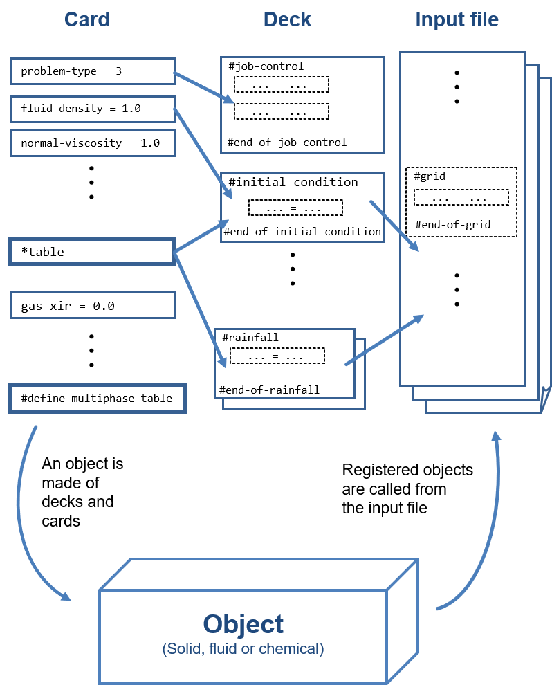
A deck is a data structure used to group some parameters together. The parameters can be card, table, import statement or other deck. groups a set of cards. The main input file is created as a combination of decks. Attributes that can be called from the deck depend on the type of object.
Fig. 4.1 represents a deck object and shows the relationship between the object and the main input file.
Note that you cannot use the same deck more than one time in the main input file.
The identifier # is a deck marker. When #
is followed by a name, it starts the deck. When it is followed by
end-of- followed by the name of the deck, it closes the
deck.
Example
#region! start of the deck
.... ... ....
.... ... ....
#end-of-region! end of the deck
Input by card (=)
Each parameter is defined in a data structure called “cards”. It is the smallest data structure of the card input format. The cards are permutable, selected by the user among the available cards in each deck. The list of cards available for each deck is predefined and depends on the deck; the order of the cards inside of a deck is arbitrary.
A single parameter is set up using a ‘card’. In a deck of settings, a parameter is set up by card with the syntax:
name-of-the-parameter = valueA value can be a single value (integer, float, string, path) or a list of values.
Input by table (*table)
Some decks accept parameters to be set up in table format. This
format is convenient to set up a group of parameters in a compact form.
The marker of a table format input is *table.
In the table format (*table), one must enter the header
of the table followed by the data. See the example below and also
Table 10.1.
In the following example, the fluid properties of gas phase and water
phase are set up in *table format.
Example:
#fluid
    #properties
        *table
            fluid-phase method-pvt  normal-fvf compressibility normal-viscosity viscosity-increment density
            water       equation    1.0        0.0             1.0              0.0                 1.0
            gas         value       n.a.       n.a.            n.a.             n.a.                1.0
    #end-of-properties
#end-of-fluid
Input by sequence of
values (*sequence-)
An input by sequence is specified with one of the markers
*sequence-cell, *sequence-side or
*sequence-cell-surface followed by a list of value
separated by space. The list of values must follows the sequence defined
by the grid input information. In case of sequence-cell,
the list must contains one value per cell. In case of
sequence-side, the list includes one value for each side of
each cell, hence six times the number of cells. In case of
sequence-cell-surface, the list must contains as many
values as a layer of the grid (fixed K value).
Dotted card (.)
Some decks allow the parameters related to fluid and region to be input using a dotted syntax. The part of the card before the dot define the deck name and the part of the card after the dot define the card name. Depending on the deck, the left part of the special card could be a region name or a fluid name. Then, the property of that region or fluid to be set up is indicated after the dot. The following examples show the field setting for the fluid (example 1) and for a region (example 2). Note that this syntax is equivalent to a deck but with an inline notation where each card is added to the deck as their order of appearance.
Example 1
water.compressibility = 1.E-5
water.viscosity = 1.E0
Example 2
sandgravel.effective-porosity = 0.35Objects (in deck #store)
Definition
An object defines a collection of data describing a specific type of entity. The type of an object can be Solid, fluid, or chemical substances. The attributes of each type differ and are partly listed below:
Solid objects Solid objects requires setting up the absolute permeability and a set of parameters that characterize the solid phase media, such as the effective porosity and the density.
Fluid objects The fluid object requires a set of fluid properties such as the viscosity, the density and the specific heat capacity.
Chemical substance objects The chemical object requires setting up the solubility, the molecular diffusion coefficients, and a set of physical properties of saturated steam.
Optional parameters and values can be gathered in objects. The available parameters depend on the type of object. An object can collects different kind of data such as experimental data and in situ data, and therefore can be used to manage data storage.
Furthermore, an object is independent from the execution of a calculation job.
If an object file is defined, data from the object will be used; if no object file is defined, the values defined in the main input file or the default values will be used for the calculation.

Usage
When solid or fluid object are defined, it is possible to use them for assigning the cards. To do this, the card is set equal to a special value that include the name of the object followed by a dot and the name of the property to by used.
The parameter of the decks #solid and
fluid>properties can be set up this way.
Example 1
water = object.fluid.groundwater.AllIn this example, all the properties of the fluid water
are assigned to the properties defined in the object
groundwater.
Example 2
loam.absolute-permeability = object.solid.silt.absolute-permeabilityIn this example, the absolute permeability of the region
loam is assigned to the absolute permeability defined in
the object silt
List of GETFLOWS cards, decks and objects
As stated previously, GETFLOWS input settings consist of objects, decks and cards. A card is necessary included in a deck; a deck can be written directly in the input file or via an object. Fig. 5.1 shows the structure of the input file.
Only the decks required for a given analysis have to be set up; the content of the input file may vary depends on the type of analysis. Although the pre-processor should accept decks in any order, it is recommended for keep the default order of decks as descibed in this document.
The table Table 5.1 lists the decks available for the water-gas two-phase flow analysis. There are three kinds of decks, depending on their usage: required, default or optional. Required mark indicate a deck that must be set up, otherwise an error message will occur. Default mark indicates that default settings will be used if the deck is not defined. Option mark indicates optional deck that may or may not be used.
The tables Table 5.3-5.10 show the cards available for each deck in a water-gas two-phase flow analysis. As same as for the decks list of Table 5.1, each card is classified into one of the three categories: required, default or optional. In case of usage the data from an object, the data can be called from a deck. See also the decks fluid-properties and solid-properties.
| Decks | Subdecks | Required | Default | Optional |
|---|---|---|---|---|
#context |
✓ | |||
#design |
#grid | ✓ | ||
| #region | ✓ | |||
| #alias-region | ✓ | |||
| #split-region | ✓ | |||
| #latitude-cell-center | ✓ | |||
#control |
#job | ✓ | ||
| #solver | ✓ | |||
| #timestep | ✓ | |||
| #flow-type | ✓ | |||
#condition |
#standard | ✓ | ||
| #initial | ✓ | |||
| #hydrostatic | ✓ | |||
| #adjust>parameter | ✓ | |||
| #adjust>waterlevel | ✓ | |||
| #adjust>cav | ✓ | |||
| #adjust>prmch | ✓ | |||
#fluid |
#properties | ✓ | ||
| #pressure-volume-temperature | ✓ | |||
#solid |
#effective-porosity | ✓ | ||
| #absolute-permeability | ✓ | |||
| #abs-perm-factor | ✓ | |||
| #manning-coefficient | ✓ | |||
| #compressibility | ✓ | |||
| #define-correlation | ✓ | |||
| #assign-correlation | ✓ | |||
| #irreducible-saturation | ✓ | |||
| #bulk-constant | ✓ | |||
#land |
#rainfall | ✓ | ||
| #evapotranspiration | ✓ | |||
| #soil-evaporation | ✓ | |||
| #well-operation | ✓ | |||
| #lsm-rainfall | ✓ | |||
| #lsm-wind-speed | ✓ | |||
| #lsm-daylight-hour | ✓ | |||
| #lsm-relative-humidity | ✓ | |||
| #lsm-albedo | ✓ | |||
| #lsm-storage | ✓ | |||
| #lsm-air-temperature | ✓ | |||
#output |
#outfile | ✓ | ||
| #outlist | ✓ | |||
| #inspect-volumeflux | ✓ | |||
| #inspect-fluidmass | ✓ | |||
| #inspect-waterlevel | ✓ | |||
| #inspect-variable | ✓ |
| Deck | Card | Required | Default (default value) | Optional |
|---|---|---|---|---|
#context |
title | ✓ | ||
| date | ✓ | |||
| author | ✓ |
| Deck | Card | Required | Default (default value) | Optional |
|---|---|---|---|---|
#linear-solver |
order | ✓ (AUT) | ||
| exclude-cell | ✓ (ON) | |||
| nxitr | ✓ (20) | |||
| north | ✓ (5) | |||
| rnorm | ✓ (-1.E-12) | |||
| nl-max-iteration | ✓ (10) | |||
| nl-epsilon | ✓ (1.0E-10) | |||
| nl-tolerance | ✓ (1.0E-6) | |||
| dumping-tolerance-coefficient | ✓ (0.0) | |||
| dumping-coefficient | ||||
| dumping-start-iteration | ||||
| slp-iteration | ✓ (2) | |||
| slp-tolerance | ✓ (1.0E-8) | |||
#primary-variable |
min-value | ✓ (PG=-1.E4(ksc); SW=0.0(farc.)) | ||
| max-value | ✓ (PG=1.E4(ksc); SW=1.0(farc.)) | |||
#timestep |
automatic | ✓ (ON) | ||
| time-unit | ✓ (DAY) | |||
| start-time | ✓ (0.0) | |||
| end-time | ✓ (1.E30) | |||
| ndt | ✓ (100,000) | |||
| dt0 | ✓ (1.E-2) | |||
| dtmax | ✓ (1.E12) | |||
| rate | ✓ (1.2) | |||
| convergence | ✓ | |||
| ntim | ✓ | |||
| dtim | ✓ | |||
#job |
problem-type | ✓ | ||
| runtype | ✓ (Run) | |||
#flow-type |
flow-type | ✓ |
| Deck | Setting | Required | Default | Options |
|---|---|---|---|---|
#fluid |
#properties |
✓ | ||
#pressure-volume-temperature |
✓ | |||
#properties |
normal-fvf | ✓ | ||
| fluid-compressibility | ✓ | |||
| normal-viscosity | ✓ | |||
| viscosity-increment | ✓ | |||
| fluid-density | ✓ | |||
| method-pvt | ✓ | |||
#pressure-volume-temperature |
pressure | ✓ | ||
| water-fvf | ✓ | |||
| gas-fvf | ✓ | |||
| water-viscosity | ✓ | |||
| gas-viscosity | ✓ |
| Deck | Card | Required | Default | Options |
|---|---|---|---|---|
#standard |
standard-pressure | ✓ (1.0033) | ||
| gravity | ✓ (9.80665) | |||
#initial |
pressure | ✓ | ||
| water-saturation | ✓ | |||
#hydrostatic |
reference-layer | ✓ | ||
| reference-point | ✓ | |||
| elevation | ✓ | |||
| density | ✓ | |||
| xopt | ✓ | |||
| reference-pressure | ✓ | |||
| reference-pc | ✓ |
| Deck | Card | Required | Default | Options |
|---|---|---|---|---|
#effective-porosity |
effective-porosity | ✓ | ||
#absolute-permeability |
file-import-cell-or-side | ✓ | ||
| abs-perm | ✓ | |||
| abs-perm-i- | ✓ | |||
| abs-perm-i+ | ✓ | |||
| abs-perm-j- | ✓ | |||
| abs-perm-j+ | ✓ | |||
| abs-perm-k- | ✓ | |||
| abs-perm-k+ | ✓ | |||
#abs-perm-factor |
abs-perm-factor-water | ✓ (1.0) | ✓ | |
| abs-perm-factor-gas | ✓ (1.0) | ✓ | ||
#manning-coefficient |
model | ✓(to add) | ||
| manning | ✓ | |||
| manning-i- | ✓ | |||
| manning-i+ | ✓ | |||
| manning-j- | ✓ | |||
| manning-j+ | ✓ | |||
#compressibility |
compressibility | ✓ | ||
#define-correlation |
mpf-name | ✓ | ||
| system | ✓ | |||
| direction | ✓ | |||
| saturation | ✓ | |||
| pc | ✓ | |||
| kr-water | ✓ | |||
| kr-napl | ✓ | |||
| kr-water-h | ✓ | |||
| kr-napl-h | ✓ | |||
| kr-water-u | ✓ | |||
| kr-napl-u | ✓ | |||
| kr-water-d | ✓ | |||
| kr-napl-d | ✓ | |||
#assign-correlation |
lg-pc-table | ✓ | ||
| lg-kr-table | ✓ | |||
| lg-kr-table-horizontal | ✓ | |||
| lg-kr-table-up | ✓ | |||
| lg-kr-table-down | ✓ | |||
| wn-kr-table | ✓ | |||
| wn-kr-table-horizontal | ✓ | |||
| wn-kr-table-up | ✓ | |||
| wn-kr-table-down | ✓ | |||
#irreducible-saturation |
water-xir | ✓ | ||
| gas-xir | ✓ |
| Deck | Card | Required | Default | Optional |
|---|---|---|---|---|
#grid |
imax | ✓ | ||
| jmax | ✓ | |||
| kmax | ✓ | |||
#region |
- | ✓ | ||
#alias-region |
(alias-name) | ✓ | ||
#split-region |
regions | ✓ | ||
#latitude-cell-center |
- | ✓ |
| Deck | Card | Required | Default | Optional |
|---|---|---|---|---|
fluid>properties |
normal-fvf | ✓ | ||
| compressibility | ✓ | |||
| normal-viscosity | ✓ | |||
| viscosity-increment | ✓ | |||
| density | ✓ | |||
| method-pvt | ✓ |
| Deck | Card | Required | Default | Optional |
|---|---|---|---|---|
#rainfall |
time-unit | ✓ (DAY) | ✓ | |
| start-time | ✓ | |||
| end-time | ✓ | |||
| rain-unit | ✓ | |||
| component | ✓ | |||
| flux | ✓ | |||
#evapotranspiration |
time-unit | ✓ (DAY) | ✓ | |
| start-time | ✓ | |||
| end-time | ✓ | |||
| pet-unit | ✓ | |||
| pet | ✓ | |||
| soil-evaporation | ✓ | |||
#soil-evaporation> |
water-saturation | ✓ | ||
#define-efficiency |
efficiency | ✓ | ||
#adjust-parameter |
time-unit | ✓ (DAY) | ✓ | |
| start-time | ✓ | |||
| end-time | ✓ | |||
| region | ✓ | |||
| i-min | ✓ | |||
| i-max | ✓ | |||
| j-min | ✓ | |||
| j-max | ✓ | |||
| k-min | ✓ | |||
| k-max | ✓ | |||
| Pg-start | ✓ | |||
| Sw-start | ✓ | |||
| rs-start | ✓ | |||
| pcc-start | ✓ | |||
| sg-start | ✓ | |||
| ra-start | ✓ | |||
| Pg-end | ✓ | |||
| Sw-end | ✓ | |||
| rs-end | ✓ | |||
| pcc-end | ✓ | |||
| sg-end | ✓ | |||
| ra-end | ✓ | |||
| water-table-water-type | ✓ | |||
| water-table-start | ✓ | |||
| water-table-end | ✓ | |||
| water-table-datum | ✓ | |||
| effective-porosity | ✓ | |||
| abs-perm | ✓ | |||
| abs-perm-i- | ✓ | |||
| abs-perm-i+ | ✓ | |||
| abs-perm-j- | ✓ | |||
| abs-perm-j+ | ✓ | |||
| abs-perm-k- | ✓ | |||
| abs-perm-k+ | ✓ | |||
| abs-perm-in | ✓ | |||
| abs-perm-in-i- | ✓ | |||
| abs-perm-in-j- | ✓ | |||
| abs-perm-in-k- | ✓ | |||
| abs-perm-interior | ✓ | |||
| abs-perm-interior-i- | ✓ | |||
| abs-perm-interior-i+ | ✓ | |||
| abs-perm-interior-j- | ✓ | |||
| abs-perm-interior-j+ | ✓ | |||
| abs-perm-interior-k- | ✓ | |||
| abs-perm-interior-k+ | ✓ | |||
| abs-perm-out | ✓ | |||
| abs-perm-out-i- | ✓ | |||
| abs-perm-out-i+ | ✓ | |||
| abs-perm-out-j- | ✓ | |||
| abs-perm-out-j+ | ✓ | |||
| abs-perm-out-k- | ✓ | |||
| abs-perm-out-k+ | ✓ | |||
| manning | ✓ | |||
| manning-i- | ✓ | |||
| manning-i+ | ✓ | |||
| manning-j- | ✓ | |||
| manning-j+ | ✓ | |||
| manning-in | ✓ | |||
| manning-in-i- | ✓ | |||
| manning-in-j- | ✓ | |||
| manning-in-k- | ✓ | |||
| manning-interior | ✓ | |||
| manning-interior-i- | ✓ | |||
| manning-interior-i+ | ✓ | |||
| manning-interior-j- | ✓ | |||
| manning-interior-j+ | ✓ | |||
| manning-interior-k- | ✓ | |||
| manning-interior-k+ | ✓ | |||
| manning-out | ✓ | |||
| manning-out-i- | ✓ | |||
| manning-out-i+ | ✓ | |||
| manning-out-j- | ✓ | |||
| manning-out-j+ | ✓ | |||
| manning-out-k- | ✓ | |||
| manning-out-k+ | ✓ | |||
| compressibility | ✓ | |||
| water-xir | ✓ | |||
| gas-xir | ✓ | |||
| napl-xir | ✓ | |||
| lg-pc-table | ✓ | |||
| lg-kr-table | ✓ | |||
| lg-kr-table-horizontal | ✓ | |||
| lg-kr-table-up | ✓ | |||
| lg-kr-table-down | ✓ | |||
| wn-pc-table | ✓ | |||
| wn-kr-table | ✓ | |||
| wn-kr-table-horizontal | ✓ | |||
| wn-kr-table-up | ✓ | |||
| wn-kr-table-down | ✓ | |||
#well-operation |
time-unit | ✓ (DAY) | ✓ | |
| start-time | ✓ | |||
| end-time | ✓ | |||
| wellhead-i | ✓ | |||
| wellhead-j | ✓ | |||
| wellhead-k | ✓ | |||
| direction | ✓ | |||
| screen | ✓ | |||
| radius | ✓ | |||
| control-type | ✓ | |||
| flowrate | ✓ | |||
| wellbtm- elevation | ✓ | ✓ | ||
| wellbtm-pressure | ✓ | |||
| well-fluid | ✓ | |||
| well-index | ✓ | ✓ |
| Deck | Card | Required | Default | Optional |
|---|---|---|---|---|
#outfile |
main | ✓ | ||
| check-list | ✓ | |||
| convergence-monitoring | ✓ | |||
| restarting-binary | ✓ | |||
| interface-velocity | ✓ | |||
| rainfall-binary | ✓ | |||
| evaporation | ✓ | |||
| evaporation-binary | ✓ | |||
| adjust-waterlevel | ✓ | |||
| variables-change | ✓ | |||
| well-operation | ✓ | |||
| volumeflux | ✓ | |||
| fluidmass | ✓ | |||
| waterlevel | ✓ | |||
| variables | ✓ | |||
| export | ✓ | |||
| file | ✓ | |||
| step | ✓ (1) | ✓ | ||
| outfolder | ✓ | ✓ | ||
#outlist |
order | ✓ (XYZ) | ✓ | |
| main-file | ✓ | |||
| check-list | ✓ | |||
#inspect-volumeflux |
group | ✓ | ||
| i-min | ✓ | |||
| i+max | ✓ | |||
| j-min | ✓ | |||
| j+max | ✓ | |||
| k-min | ✓ | |||
| k+max | ✓ | |||
| output | ✓ | |||
#inspect-fluidmass |
region | ✓ | ||
| i-min | ✓ | |||
| i+max | ✓ | |||
| j-min | ✓ | |||
| j+max | ✓ | |||
| k-min | ✓ | |||
| k+max | ✓ | |||
| porosity-min | ✓ (-10.0) | ✓ | ||
| porosity-max | ✓ (10.0) | ✓ | ||
| saturation-min | ✓ (-10.0) | ✓ | ||
| saturation-max | ✓ (10.0) | ✓ | ||
#inspect-waterlevel |
i-min | ✓ | ||
| i+max | ✓ | |||
| j-min | ✓ | |||
| j+max | ✓ | |||
| k-min | ✓ | |||
| k+max | ✓ | |||
| option | ✓ | |||
#inspect-variable |
i | ✓ | ||
| j | ✓ | |||
| k | ✓ | |||
| name | ✓ | |||
#inspect-chemical |
i | ✓ | ||
| j | ✓ | |||
| k | ✓ | |||
| name | ✓ | |||
#inspect-budget |
region | ✓ | ||
| group | ✓ |
The default output file contains the primary variables values on the entire computational grid. The primary variables depend on the type of simulations, as detailed in . For a water-gas two-phase flow analysis, the outputs at each cell are the air pressure and the aqueous phase saturation. The pressure of the aqueous phase and the gas phase saturation are not written directly to the output file. The aqueous phase pressure is equal to the gas phase pressure minus the capillary pressure. The gas phase saturation is equal to one (‘1’) minus the aqueous phase saturation. To output specific values such as flow rate of aqueous through a given cell, specific instruction must be added to the main input file.
| Pres. | Pres. | Pres. | Sat. | Sat. | Sat. | Conc. | Conc. | Conc. | Terrain elevation | Temp. | Temp. | |
|---|---|---|---|---|---|---|---|---|---|---|---|---|
| Aqueous phase | Gas phase | NAPL phase | Aqueous phase | Gas phase | NAPL phase | Aqueous phase | Gas phase | Swimming sand | Fluid phase | Solid phase | ||
| Water-gas two-phase flow analysis | ✓ | ✓ | ||||||||||
| Density flow analysis | ✓ | ✓ | ✓ | |||||||||
| Water-gas-NAPL three-phase flow analysis | ✓ | ✓ | ✓ | ✓ | ✓ | ✓ | ||||||
| Analysis of reactive mass transport | ✓ | ✓ | ||||||||||
| Hydrothermal transport system coupled analysis | ✓ | ✓ | ✓ | ✓ | ||||||||
| Wed sediment landform coupled analysis | ✓ | ✓ | ✓ | ✓ |
Input by region or by ijk value
The following table list the allowed entries of a table along with their description.
| Header keyword | Type | Description | Default |
|---|---|---|---|
| region | string | region name | No |
| i-min | string | Range of cell number: I min. | No |
| i-max | string | Range of cell number: I max. | No |
| j-min | string | Range of cell number: J min. | No |
| j-max | string | Range of cell number: J max. | No |
| k-min | string | Range of cell number: K min. | No |
| k-max | string | Range of cell number: K max. | No |
There is two methods of allocation of properties to a cell or a group
of cell: in case of region, the properties are allocated to
groups of cells designed by their region name (see also design>region deck and #alias-region. In the other case,
two integers for each direction defines the numbers of cells in the
group.
| Deck | SubDeck | First column | Following columns (arbitrary order) |
|---|---|---|---|
| #control | #primary-variable | primary-variable | min-value |
| max-value | |||
| epsilon | |||
| slp-tolerance | |||
| tolerance | |||
| #control | #timestep | ntim | dtim |
| #control | #flow-type | region, ijk | flowtype |
| #fluid | #properties | fluid-phase | normal-fvf |
| fluid-compressibility | |||
| normal-viscosity | |||
| viscosity-increment | |||
| fluid-density | |||
| method-pvt | |||
| #fluid | #pressure-volume-temperature | pressure | water-fvf |
| gas-fvf | |||
| water-viscosity | |||
| gas-viscosity | |||
| #condition | #initial | region, ijk | Pg |
| Sw | |||
| #condition | #hydrostatic | region, ijk | reference-layer |
| reference-point | |||
| elevation | |||
| density | |||
| xopt | |||
| reference-pressure | |||
| reference-pc | |||
| water-type | |||
| #solid | #effective-porosity | region, ijk | effective-porosity |
| #solid | #absolute-permeability | region, ijk | abs-perm |
| abs-perm-i- | |||
| abs-perm-i+ | |||
| abs-perm-j- | |||
| abs-perm-j+ | |||
| abs-perm-k- | |||
| abs-perm-k+ | |||
| #solid | #abs-perm-factor | region, ijk | abs-perm-factor-water |
| abs-perm-factor-gas | |||
| #solid | #manning-coefficient | region, ijk | manning |
| manning-i- | |||
| manning-i+ | |||
| manning-j- | |||
| manning-j+ | |||
| #solid | #compressibility | region, ijk | compressibility |
| #multiphase | #define-correlation | saturation | capillary-pressure |
| kr-water | |||
| kr-napl | |||
| kr-water-h | |||
| kr-napl-h | |||
| kr-water-u | |||
| kr-napl-u | |||
| kr-water-d | |||
| kr-napl-d | |||
| #multiphase | #assign-correlation | region, ijk | lg-capillary-pressure |
| lg-kr-table | |||
| lg-kr-table-horizontal | |||
| lg-kr-table-up | |||
| lg-kr-table-down | |||
| #solid | #irreducible-saturation | region, ijk | water-xir |
| gas-xir | |||
| #fluid | #properties | fluid | normal-fvf |
| fluid-compressibility | |||
| normal-viscosity | |||
| viscosity-increment | |||
| fluid-density | |||
| method-pvt |
Context
This deck is used to describe the context of the simulation. It contains only four cards: title, author, project and date (what, who, where and when).
Description
Define the ongoing simulation, including for instance the title of the simulation, the date and the name of the author.
Identifier
| Starting deck | #context |
| Ending deck | #end-of-context |
List of cards
| Card name | Type | Description | Default |
|---|---|---|---|
| title | string | A string used to define the title of the analysis | No |
| date | string | A string used to define the date of the analysis | No |
| author | string | A string used to define the author’s name | No |
See also
None
Example
#context
    title = Simulation-Title
    date   = Dec24-2009
    author = Name
#end-of-context
Design
Grid
Description
Define the corner point coordinates value of the three-dimensional grid system.
Identifier
The marker of the grid deck is as below.
| Starting deck | #grid |
| Ending deck | #end-of-grid |
List of cards
| Card name | Type | Description | Default |
|---|---|---|---|
| imax | integer | Number of grid cells in the I-direction | No |
| jmax | integer | Number of grid cells in the J-direction | No |
| kmax | integer | Number of grid cells in the K-direction | No |
Grid numbering of the three-dimensional grid system is defined in a three axis system I-J-K that reproduce as much as possible the Cartesian coordinate system X-Y-Z (see Fig. 7.1). Usually, the directions I, J define the plane XY and the direction K is the depth axis (Z axis). The total number of cells in each direction I,J,K is noted respectively NX, NY and NZ. The total number of grid cells is calculated as follows:
NNBLK = NX * NY * NZ.The number of corner points coordinates value in each direction I,J,K is noted respectively NXP, NYP and NZP. The relationship between the number of grid cells and the number of corner points is:
NXP = NX + 1, NYP = NY + 1, NZP = NZ + 1The total number of corner points is defined by:
nnblkp = nxp*nyp*nzpThe corner points coordinates value should be input in the following order.
- X coordinates value
- Y coordinates value
- Z coordinates value
Also each set of coordinates value should be preceded by a string indicating which coordinates value are input, usually ‘X’, ‘Y’ and ‘Z’ (see also the example).
Z-axis direction is oriented toward the decreasing elevation. So the direction of increasing coordinates is oriented toward the opposite of the elevation.
The coordinates value of the corner points should be input in an predefined order, I-J-K directions, as follows.
(1,1,1)(2,1,1)...(NXP,1,1)(1,2,1)(2,2,1)...(NXP,2,1)...(NXP,NYP,1)
(1,1,2)(2,1,2)...(NXP,1,2)(1,2,2)(2,2,2)...(NXP,2,2)...(NXP,NYP,2)
... ... ...
(1,1,NZP)(2,1,NZP)...(NXP,1,NZP)(1,2,NZP)(2,2,NZP)...(NXP,2,NZP)...(NXP,NYP,NZP)
See also
None
Example
#grid
   imax = 4
   jmax = 2
   kmax = 4
   *sequence-cell
      'X'
      0.0 1.0 2.0 3.0 4.0 0.0 1.0 2.0 3.0 4.0 0.0 1.0 2.0 3.0 4.0
      0.0 1.0 2.0 3.0 4.0 0.0 1.0 2.0 3.0 4.0 0.0 1.0 2.0 3.0 4.0
      0.0 1.0 2.0 3.0 4.0 0.0 1.0 2.0 3.0 4.0 0.0 1.0 2.0 3.0 4.0
      0.0 1.0 2.0 3.0 4.0 0.0 1.0 2.0 3.0 4.0 0.0 1.0 2.0 3.0 4.0
      0.0 1.0 2.0 3.0 4.0 0.0 1.0 2.0 3.0 4.0 0.0 1.0 2.0 3.0 4.0
      'Y'
      0.0 0.0 0.0 0.0 0.0 1.0 1.0 1.0 1.0 1.0 2.0 2.0 2.0 2.0 2.0
      0.0 0.0 0.0 0.0 0.0 1.0 1.0 1.0 1.0 1.0 2.0 2.0 2.0 2.0 2.0
      0.0 0.0 0.0 0.0 0.0 1.0 1.0 1.0 1.0 1.0 2.0 2.0 2.0 2.0 2.0
      0.0 0.0 0.0 0.0 0.0 1.0 1.0 1.0 1.0 1.0 2.0 2.0 2.0 2.0 2.0
      0.0 0.0 0.0 0.0 0.0 1.0 1.0 1.0 1.0 1.0 2.0 2.0 2.0 2.0 2.0
      'Z'
      -2. -2. -2. -2. -2. -2. -2. -2. -2. -2. -2. -2. -2. -2. -2.
      -1. -1. -1. -1. -1. -1. -1. -1. -1. -1. -1. -1. -1. -1. -1.
      0.0 0.0 0.0 0.0 0.0 0.0 0.0 0.0 0.0 0.0 0.0 0.0 0.0 0.0 0.0
      1.0 1.0 1.0 1.0 1.0 1.0 1.0 1.0 1.0 1.0 1.0 1.0 1.0 1.0 1.0
      2.0 2.0 2.0 2.0 2.0 2.0 2.0 2.0 2.0 2.0 2.0 2.0 2.0 2.0 2.0
#end-of-grid
Region
Description
Define the region names and the set of grid cells that belong to each region.
Identifier
| Starting deck | #region |
| Ending deck | #end-of-region |
List of cards
| Card name | Type | Description | Default |
|---|---|---|---|
| gfbase-format | string | if blk: the file imported in
the *import-gfbase statement should be a blk file |
- |
if region: the file imported
in the *import-gfbase statement should be a region
file |
|||
This card is used only if
*import-gfbase is used. |
List of column in table
| Card name | Type | Description | Default |
|---|---|---|---|
| i-min | integer | First cell of the region in the I direction | - |
| i-max | integer | Last cell of the region in the I direction | - |
| j-min | integer | First cell of the region in the J direction | - |
| j-max | integer | Last cell of the region in the J direction | - |
| k-min | integer | First cell of the region in the K direction | - |
| k-max | integer | Last cell of the region in the K direction | - |
The name of the region is defined as the table name (a string within
| following the *table statement. Ex:
*table |atmosphere|
A region is a name assigned to a set of grid cells. The cells of each region are identified with their IJK number. Regions such as geological layer, land use, or boundary conditions can be commonly-referred in the overall input file, to facilitate the setting of input conditions.
See also
#[alias-region], design>split-region
Example
Example 1 (set up with table and importing):
#region
    *table |Atmosphere|
        i-min i-max j-min j-max k-min k-max
        1     12    1     1     1     1
    *table |Surface|
        i-min i-max j-min j-max k-min k-max
        1     12    1     1     2     2
    *table |UnderGround|
        i-min i-max j-min j-max k-min k-max
        12    12    1     1     4     4
        11    11    1     1     3     3
    *import
       <region.gfcard>
#end-of-region
Example 2 (set up by importing a gfbase blk file):
#region
    gfbase-format = blk
    *import-gfbase
        <ext-gfbase/blk.001>
#end-of-region
Example 3 (set up by importing a gfbase region file):
#region
    gfbase-format = region
    *import-gfbase
        <ext-gfbase/reg.001>
#end-of-region
Alias-region
Description
Define the region alias (group of regions).
Identifier
| Starting deck | #alias-region |
| Ending deck | #end-of-alias-region |
List of cards
| Card name | Type | Description | Default |
|---|---|---|---|
| name | string | A string defining the name of the alias | - |
| region-list | list | A list of strings defining the name of the regionsbelonging to the alias | - |
| *import | import | Use an *import section to add
alias from an external file |
Note that using an *import section, it is possible to
include alias from an external file.
See also
design>region, design>split-region.
Example
#alias-region
    All = Atmosphere Surface UnderGround
    Boundary = UpStream DownStream
#end-of-alias-region
Split-region
Description
Define the partial region for region decomposition method. Note:
split-region was named Solver Split in
previous version of GETFLOWS.
Identifier
| Starting deck | #split-region |
| Ending deck | #end-of-split-region |
List of cards
| Card name | Type | Description | Default |
|---|---|---|---|
| region-list | string | List of regions where to apply the region
decomposition method (names of regions have to be defined in the
design>region deck) |
- |
| orders | string | Storage order of the Jacobian determinant passed to the linear solver (input to the number of regions defined by region card) | See below |
This deck lists the regions where to distribute the computation tasks
(card regions). In the boundary of the sub-regions (ghost zone), the
primary variables (pressure, saturation) are shared. Then, the numeric
solution for all regions is given. The sub-region should be defined in
design>region and design>alias-region
decks. Each sub-region can re-define the storage order of the Jacobian
determinant defined by #solver (card ORDERS). Unless
re-defined in this deck, the configuration of #solver is
valid in all sub-regions.
See also
control>linear-solver,
control>nonlinear-solver,
design>region, design>alias-region
Example
#split-region
    region-list = surface soil-a soil-b
    orders = XYZ ZXY ZXY
#end-of-split-region
Latitude of cell center
Description
Define the latitude of the center of each cell. Use the gfbase format.
Identifier
| Starting deck | #latitude-cell-center |
| Ending deck | #end-of-latitude-cell-center |
List of cards
None
List of column in table
None
See also
None
Example
#latitude-cell-center
    *import-gfbase
        <ext-gfbase/lat.001>
#end-of-latitude-cell-center
Control
The control deck is used to set up the parameters that
control the behaviour of the simulator. The parameters are grouped into
severals decks: the job deck define the type of simulation,
the linear and non-linear solver decks set up the solver parameters, the
primary-variable deck contains the range of each variables and the
solver parameters realted to the primary variables, the timestep deck
includes the parameters defining the time properties of the solver, the
flow-type and nb-equation deck define the type and the number of
equation to be solve in each cell, the lsm-control deck set up the
parameters of the land-surface model.
Job
Description
Define several general settings related to the type of simulation conducted: analysis type, execution mode, option for the advection model, fluid component system, etc.
Identifie
| Starting deck | #job |
| Ending deck | #end-of-job |
List of cards
| Card name | Type | Description | Default value |
|---|---|---|---|
| problem-type | integer | Integer defining the type of problem solved (c.f. Table 8.2) | No |
| runtype | string | Execution type | Run |
| if Run: Normal run | |||
| if Post: Post-processing run. Using the previously computed results, it only create the requested output files. | |||
| advection (not used) | string | Advection options | Transient |
| if Stationary: Steady flow velocity distribution | |||
| if Transient: Unsteady flow velocity distribution |
Notes:
- The fluid component systems that fixes the number of equations to be solved per cell (corresponding to the number of primary variables) is determined by the selected problem type (cf. Table 8.2).
- In the water-gas two-phases flow analysis, GETFLOWS calculates the aqueous phase saturation and the gas phase pressure in every cells ; the number of equations should be nb-equation=2.
- The names of the fluid phase are fixed depending on the problem-type (see Table 8.2). In GETFLOWS, there is a maximum of three phases: Aqueous phase, gas phase and NAPL phase. The fluid phase names are used when setting the fluid properties.
See also
#pressure-volume-temperature,
#normal-fvf, #normal-viscosity, #viscosity-increment, #method-pvt, #fluid>properties
Example
#job
   problem-type = 3
   runtype    = Run
#end-of-job| Problem type | Nb equation | Nb phase | Nb chemical | Nb chemical liquid | Nb chemical gas | Fluid phase | Fluid component | Job type | Landform change | Heat transport | Fluid-solid heat | THMC | Primary variable |
|---|---|---|---|---|---|---|---|---|---|---|---|---|---|
| 1 | 1 | 1 | 0 | 0 | 0 | water | N.A. | N.A. | No | No | N.A. | H | N.A. |
| 2 | 1 | 1 | 0 | 0 | 0 | gas | N.A. | N.A. | No | No | N.A. | H | N.A. |
| 3 | 2 | 2 | 0 | 0 | 0 | water,gas | water,gas | flows | No | No | N.A. | H | Pg,Sw |
| 4 | 3 | 2 | 1 | 1 | 0 | water,gas | water,gas | flows | No | No | N.A. | HC | Pg,Sw,rs1 |
| 5 | 3 | 3 | 1 | 1 | 0 | water,gas,napl | water,gas,napl,rs1 | flows | No | No | N.A. | HC | pn,sg,Sw,rs1 |
| 6 | 5 | 3 | 2 | 1 | 1 | water,gas,napl | water,gas,napl,rs1,rg1 | flows | No | No | N.A. | HC | pn,sg,Sw,rs1,rg1 |
| 7 | 2 | 2 | 1 | 1 | 0 | water,gas | water,gas,rs1 | flows | No | No | N.A. | HC | Pg,Sw,rs1 |
| 8 | 2 | 2 | 2 | 1 | 1 | water,gas | rs1,rg1 | trans | No | No | N.A. | HC | rs1,rg1 |
| 9 | 5 | 3 | 2 | 1 | 1 | water,gas,napl | water,gas,napl,rs1,rg1 | flows | No | No | N.A. | HC | Pg,sg,Sw,rs1,rg1 |
| 10 | 4 | 2 | 0 | 0 | 0 | water,gas | water,gas | flows | No | Yes | different | TH | Pg,Sw,tf,ts |
| 11 | 4 | 2 | 2 | 2 | 0 | water,gas | water,gas,rs1,rs2 | flows | No | No | N.A. | HC | Pg,Sw,rs1,rs2 |
| 12 | 5 | 2 | 3 | 3 | 0 | water,gas | water,gas,rs1,rs2,rs3 | flows | No | No | N.A. | HC | Pg,Sw,rs1,rs2,rs3 |
| 13 | 2 | 2 | 2 | 2 | 0 | water,gas | rs1,rs2 | trans | No | No | N.A. | HC | rs1,rs2 |
| 14 | 6 | 3 | 3 | 3 | 0 | water,gas,napl | water,gas,napl,rs1,rs2,rs3 | flows | No | No | N.A. | HC | pn,sg,Sw,rs1,rs2,rs3 |
| 15 | 5 | 2 | 1 | 1 | 0 | water,gas | water,gas,rs1 | flows | No | Yes | different | THC | Pg,Sw,rs1,tf,ts |
| 16 | N.A. | N.A. | N.A. | N.A. | N.A. | N.A. | N.A. | N.A. | No | N/A | N.A. | N.A. | N.A. |
| 17 | 3 | 2 | 3 | 3 | 0 | water,gas | rs1,rs2,rs3 | trans | No | Yes but not used | N.A. | THC | rs1,rs2,rs3 |
| 18 | N.A. | N.A. | N.A. | N.A. | N.A. | N.A. | N.A. | N.A. | No | N/A | N.A. | N.A. | N.A. |
| 19 | 6 | 2 | 4 | 2 | 2 | water,gas | water,gas,rs1,rg1,rs2,rg2 | flows | No | No | N.A. | HC | Pg,Sw,rs1,rg1,rs2,rg2 |
| 20 | 1 | 2 | 1 | 1 | 0 | water,gas | rs1 | trans | No | No | N.A. | HC | rs1 |
| 21 | 4 | 2 | 2 | 1 | 1 | water,gas | water,gas,rs1,rg1 | flows | No | No | N.A. | HC | Pg,Sw,rs1,rg1 |
| 22 | 3 | 2 | 0 | 0 | 0 | water,gas | water,gas | flows | No | Yes | identical | TH | Pg,Sw,t |
| 23 | 4 | 2 | 1 | 1 | 0 | water,gas | water,gas,rs1 | flows | No | Yes | identical | THC | Pg,Sw,rs1,t |
| 24 | N.A. | N.A. | N.A. | N.A. | N.A | N.A. | N.A. | N.A. | No | N/A | N.A. | N.A. | N.A. |
| 25 | 3 | 2 | 3 | 3 | 0 | water,gas | rs1,rs2,rs3 | trans | No | No | N.A. | HC | rs1,rs2,rs3 |
| 26 | 6 | 2 | 2 | 1 | 1 | water,gas | water,gas,rs1,rg2 | flows | No | Yes | different | THC | Pg,Sw,rs1,rs2,tf,ts |
| 27 | N.A. | N.A. | N.A. | N.A. | N.A | N.A. | N.A. | N.A. | No | Yes | N.A. | N.A. | N.A. |
| 28 | 2 | 2 | 2 | 1 | 1 | water,gas | age-water | histr | No | No | N.A. | HC | age,unused |
| 29 | 2 | 2 | 0 | 0 | 0 | water,gas | water,gas | LSM | No | No | N.A. | H | Pg,Sw |
| 30 | 2 | 2 | 0 | 0 | 0 | water,gas | water,gas,sediment | sedim | Yes | No | N.A. | HM | Pg,Sw,xs |
| 31 | 2 | 2 | 0 | ICSOPT | 0 | water,gas | water,gas,sediment+rs | sedim | Yes | No | N.A. | HC | Pg,Sw,xs,rs |
| 32 | 3 | 2 | 0 | ICSOPT+1 | 0 | water,gas | water,gas,sediment+rs,rs | sedim | Yes | No | N.A. | HC | Pg,Sw,xs,rxs,rs2 |
| 33 | 3 | 2 | 3 | 3 | 0 | water,gas,rs | age-water | histr | No | No | N.A. | HC | age,unused,unused |
| 34 | 4 | 2 | 4 | 4 | 0 | water,gas | rs1,rs2,rs3,rs4 | trans | No | No | N.A. | HC | rs1,rs2,rs3,rs4 |
| 35 | 3 | 3 | 0 | 0 | 0 | water,gas,napl | water,gas,napl | flows | No | No | N.A. | HC | pn,sg,Sw |
| 36 | 8 | 3 | 4 | 2 | 2 | water,gas,napl | water,gas,napl,rs1,rg1,rs2,rg2,t | flows | No | Yes | identical | THC | pn,sg,Sw,rs1,rg1,rs2,rg2,t |
| 37 | 2 | 2 | 2 | 2 | 0 | water,gas | p1,p2 | trans | No | No | N.A. | HC | p1,p2 |
| 38 | 5 | 3 | 1 | 1 | 0 | water,gas,napl | water,gas,napl,rs1 | flows | No | Yes | identical | THC | pn,sg,Sw,rs1,t |
| 39 | 6 | 3 | 2 | 1 | 1 | water,gas,napl | water,gas,napl,rs1,rg1 | flows | No | Yes | identical | THC | pn,sg,Sw,rs1,rg1,t |
Notes:
- N.A.: Not Assigned.
- THMC: Thermal Hydrologic Mechanical Chemical processes.
- The number of equation correspond of the number of primary variable (last column).
- The number of component is the number of phase + the number of chemical species.
- When the job type is
Flow, the number of equation is the number of phase + the number of chemical. - When the job type is
Trans, the number of equation is the number of phase. - When
Heat transportis considered, two primary variables are added. - ICSOPT: number of solute under the 2-step solute computation method. ICSOPT is used as special treatment in solute transport simulation. Solute concentration, fluid pressure and saturation is usually solved simultaneously in solute transport simulation. Another solution method is incorporated into GETFLOWS, firstly, fluid pressure and saturation is solved, then only concentration is solved using calculated fluid velocity as operator split approach. ICSOPT shows number of solute in this method.
Jobtype designs the type of simulation. It is either
Flows, Trans, LSM,
Histr or Sedim.
Flows: Mass transport and fluid flow computation. Used for 3-phase 2-component flow calculations such as density and flow analysis considering the velocity field and concentration field interaction.Trans: Transport computation based on previously computed fluid flow results (FLOW option). The system uses a dilute solution without interaction velocity field and concentration field (currently not used).Sedim: Sediment transport calculation (Bed load). Consider the simultaneous interaction of suspended sediment transport and topographic change.LSM: Land Surface Model.histr: historic
List of primary-variables:
- Pg: Gas pressure (unit: kgf/cm2)
- Pn: NAPL pressure (unit: kgf/cm2)
- Sw: Water saturation (unit: None)
- Sg: Gas saturation (unit: None)
- Rs: Volume concentration of dissolved matter in the water phase (unit: None)
- Rg: Volume concentration of volatilized matter in the air phase (unit: None)
- Tf: Mean temperature of fluid phases (unit: °C)
- Ts: Solid phase thenperature (unit: °C)
- T : Mean temperature of the and solid phases (unit: °C)
- P (P1, P2) : Probability distribution (unit: None)
- Xs: Concentration of suspended sediment
- Age: Groundwater age (unit: time)
Linear solver
Description
Define the parameters of the linear solver.
Identifier
| Starting deck | #linear-solver |
| Ending deck | #end-of-linear-solver |
List of cards
| Card name | Type | Description | Default |
|---|---|---|---|
| matrix-order | string | Set up the order of storage of the Jacobian matrix passed to the linear solver. | AUT |
| = XYZ | |||
| Define the position of each coordinate in the diagonal (by deck) Jacobian matrix (Newton-Raphton iteration), from the innermost off-diagonal element (here X) to the outermost element (here Z) | |||
| The possibility are: ORDER = “XZY”, “YZX”, “YXZ”, “ZXY” and “ZYX”. | |||
| Note that in a 1D model, the Jacobian matrix is tri-diagonal (by deck), while it is penta-diagonal and hepta-diagonal in a 2D and 3D model respectively. | |||
| This parameter influcence the numerical stability of the solution. The order is usually selected so that coordinate with the higher flow is on the innermost diagonal. | |||
| = AUT: In this mode, the component of larger flow direction is automatically selected. | |||
| max-iteration (nxitr) | integer | Maximum number of iterations of the linear solver | 20 |
| north | integer | Number of orthogonal vector used in the method ORTHOMIN | 5 |
| convergence-tolerance-value (rnorm) | float | Value of the residual norm of the total area used as a convergence criterion by the linear solver. The type of residual norms is specified by the sign. If the value is positive, the relative residual norm is used; if the value is negative, the absolute residual norm is used (default setting). | -1.E-12 |
| library | string | original, MKL, Lis | original |
| method | string | GBiCGSTAB, BiCGSTAB, GCR | GBiCGSTAB |
| GBiCGSTAB.s | float | [coming soon] | 3 |
| GBiCGSTAB.L | float | [coming soon] | 3 |
| BiCGSTAB.s | float | [coming soon] | 3 |
| GCR.m | float | [coming soon] | 30 |
| preconditioner | string | GBILUp, Nest, None | GBILUp |
| GBILUp.p | float | [coming soon] | 2 |
| convergence-tolerance-method | string | ABS, RELT | ABS |
See also
Examples
Example 1
#linear-solver
   library = original    ! MKL, Lis
   method = GBiCGSTAB ! GBiCGSTAB, BiCGSTAB, GCR
   GBiCGSTAB.s = 3
   GBiCGSTAB.L = 3
   BiCGSTAB.s = 3
   GCR.m = 30
   preconditioner = GBILUp ! GBILUp, Nest, None
   GBILUp.p = 2
   matrix-order = 'XYZ'
   convergence-tolerance-method = ABS  ! ABS, RELT
   convergence-tolerance-value = 1.d-12
   max-iteration = 50

   !order = AUT      ! AUT, XYZ, XZY, YXZ, YZX, ZXY, ZYX
   !rnorm =-1.E-12
   !north = 5
   !nxitr = 20
#end-of-linear-solver
Note on versions
The gfcard input also support the version v6-x-x of GETFLOWS with the following deck:
#linear-solver
   max-iteration = 50
   rnorm = -1.e-12
   north = 10
   nxitr = 20
   order = 'XYZ'
#end-of-linear-solver
Here, the parameter rnorm can be negative. If rnorm is
positive, RELT method is used. If rnorm is negative, ABS method is
used.
Depending on the version (6-x-x or 7-x-x), the gfbase input related to the linear solver made by the card input processing is as follow.
For GF6 (version v6-x-x), the input in job file is:
'SOLVER-SETTING (rnorm,north,nxitr,XYZorder) ' -1.0d-12,3,3,3000,'ZXY'For GF7 (version v7-x-x), the input in job file is
either:
original:
'LINEAR-SOLVER-LIBRARY                       ' 'ORIGINAL'               ! 'ORG'  or 'MKL'  or 'LIS' , def.='ORG'
'LINEAR-SOLVER-METHOD                        ' 'GBiCGStab'  3  3        ! def.='GBiCGStab' 3 3
'LINEAR-SOLVER-PRECONDITIONER                ' 'GBILUp'  2              ! def.='GBILUp' 2
'LINEAR-SOLVER-MATRIX-ORDER                  ' 'XYZ'                    ! 'XYZ' or 'YXZ' or .... or 'AUT'  , def='AUT'
'LINEAR-SOLVER-CONVERGENCE-TOLERANCE         ' 'ABS'  1.d-12            ! 'ABS' or 'RELT'  , def='ABS'
'LINEAR-SOLVER-MAXIMUM-ITERATIONS            ' 50                       ! def.=50
LIS:
'LINEAR-SOLVER-LIBRARY                       ' 'LIS'                    ! 'ORG'  or 'MKL'  or 'LIS' , def.='ORG'
'LINEAR-SOLVER-MATRIX-ORDER                  ' 'XYZ'                    ! 'XYZ' or 'YXZ' or .... or 'AUT'  , def='AUT'
'LINEAR-SOLVER-CONVERGENCE-TOLERANCE         ' 'ABS'  1.d-12            ! 'ABS' or 'RELT'  , def='ABS'
'LINEAR-SOLVER-MAXIMUM-ITERATIONS            ' 50                       ! def.=50
'LINEAR-SOLVER-LIS-COMMANDLINE-OPTION        ' '-i 9 -p 2 -ilu_fill 2 -print 3'
MKL:
'LINEAR-SOLVER-LIBRARY                       ' 'MKL'               ! 'ORG'  or 'MKL'  or 'LIS' , def.='ORG'
'LINEAR-SOLVER-MATRIX-ORDER                  ' 'XYZ'               ! 'XYZ' or 'YXZ' or .... or 'AUT'  , def='AUT'
Nonlinear solver
Description
Define the parameters of the nonlinear solver.
Identifier
| Starting deck | #nonlinear-solver |
| Ending deck | #end-of-nonlinear-solver |
List of cards
| Card name | Type | Description | Default |
|---|---|---|---|
| exclude-cell | string | This option is used to force the solver to exclude the cells with large effective porosity value (greater than 1.E10). | ON |
| = ON: The option is effective (cells are excluded). | |||
| = OFF: The option is ineffective (cells are not excluded). | |||
| max-iteration | integer | Maximum number of iterations of the nonlinear calculation | 10 |
| dumping-tolerance-coefficient | float | Dumping is a convergence relaxation function. During the non-linear
iterative calculation, if the number of iterations is equal to or
greater than dumping-start-iteration, and if the maximum
change of primary variable (PV) between previous and current iteration
is equal to or less than the value tolerance*dumping, then
the PV change DX of each cell will be updated to be
DX*dumping-coefficient. |
0.0 |
| dumping-coefficient | float | See dumping-tolerance-coefficient above. |
0.7 |
| dumping-start-iteration | float | See dumping-tolerance-coefficient above. |
- |
| slp-iteration | float | Number of non-linear iterative calculation during when the SLP option is not activated. SLP can be disable by entering a number greater than the upper limit of the number of iterations of the non-linear calculation (slp-iteration >= max-iteration). | 2 |
See also
Examples
Example:
#nonlinear-solver
   max-iteration = 10
   slp-iteration = 2
   dumping-tolerance-coefficient = 1.E1
   exclude-cell = ON
#end-of-nonlinear-solver
Primary-variable
Description
Define the parameters related to the primary variables (gas pressure, water saturation, etc).
Identifier
| Starting deck | #primary-variable |
| Ending deck | #end-of-primary-variable |
List of cards
| Card name | Type | Description | Default |
|---|---|---|---|
| min-value | float | Set up the minimum value of each unknown variable | PG = - 10 4 (ksc) ; SW = 0.0 (frac.) (*) |
| max-value | float | Set up the maximum value of each unknown variable | PG =10 4 (ksc) ; SW =1.0 (frac.) (*) |
| nl-epsilon | float | Small variation of each unknown variable used to evaluate the numerical derivative of the Jacobian | 1.0E-10 for each PV |
| nl-tolerance | float | If the residual norm of the PV is lower than
nl-tolerance value, the non-linear iteration is said
converged. One value for each PV should be input. |
1.0E-6 for each PV |
| slp-tolerance | float | Value of the PV amount of change between two iterations under which the cells are excluded of the linear solver. The residual norm of the primary variables is used to determine the convergence. One value for each PV should be input. | 1.0E-8 for each PV |
(*) PG: gas phase pressure (kgf/cm2). SW: aqueous phase saturation (frac.)
Examples
Example 1: Set up by *table
#primary-variable
    *table
       primary-variable min-value  max-value nl-epsilon slp-tolerance nl-tolerance  timestep-tolerance
       PG               -1.E4      1.E4      1.E-10     1.E-7         1.E-5         1.0E-06
       SW                0.0       1.0       1.E-10     1.E-7         1.E-5         1.0E-06
    #end-of-primary-variable
Example 2: Set up by primary-variable
#primary-variable
    PG.min-value = -1.E4
    PG.max-value = 1.E4
    PG.nl-epsilon = 1.E-10
    PG.slp-tolerance = 1.E-8
    PG.nl-tolerance = 1.E-6
    PG.timestep-tolerance = 1.0E-06

    SW.min-value = 0.E0
    SW.max-value = 1.E0
    SW.nl-epsilon = 1.E-10
    SW.slp-tolerance = 1.E-8
    SW.nl-tolerance = 1.E-6
    SW.timestep-tolerance = 1.0E-06
#end-of-primary-variable
Timestep
Description
Define the time setting of the computation.
Identifier
| Starting deck | #timestep |
| Ending deck | #end-of-timestep |
List of cards
| Card name | Type | Description | Default |
|---|---|---|---|
| automatic | string | Define the computation method of the time step | ON |
if on then Automatic |
|||
if off then Fixed |
|||
| time-unit | string | Time unit | DAY |
if year then Year |
|||
if week then Week |
|||
if day then Day |
|||
if hour then Hour |
|||
if min then Minute |
|||
if sec then Second |
|||
| start-time | float or | if a float number then define the instant
when computation start (real number in unit defined by the
time-unit card). |
0.0 |
| string | if hot-start then the first
line of the file given in the card *sequence-cell of the
deck condition>initial is used as starting time. |
||
| end-time | float | Define the instant when computation stop | 1.E30 |
| ndt | integer | Define the maximum number of time steps | 1.E5 |
| dt0 | float | Define the initial time step (can be used
only when automatic = ON) |
1.E-2 |
| dtmax | float | Define the greatest time step (can be used
only when automatic = ON) |
1.E10 |
| rate | float | Define the multiplicative coefficient
applied on the current time step to define the new time step (can be
used only when automatic = ON) |
1.2 |
| timestep-convergence | float | Define the relaxation value used to
determine the convergence of the linear solver. The numerical solution
is assumed to have converged when the decrease of the residual norm at
each iteration falls below this value. The range is 0 to 1 (can be used
only when automatic = ON). |
0 |
| ntim | integer | Define the number of steps with the
corresponding DTIM time step (used when
automatic = OFF). |
None |
Note: this card is available only as a
*table |manual-timestep| format entry (c.f. example 2
below). |
|||
| dtim | float | Define the fixed time step used for the
corresponding NTIM number of time steps (only used when
automatic = OFF). |
None |
Note: this card is available only as a
*table |manual-timestep| format entry (c.f. example 2
below). |
Notes:
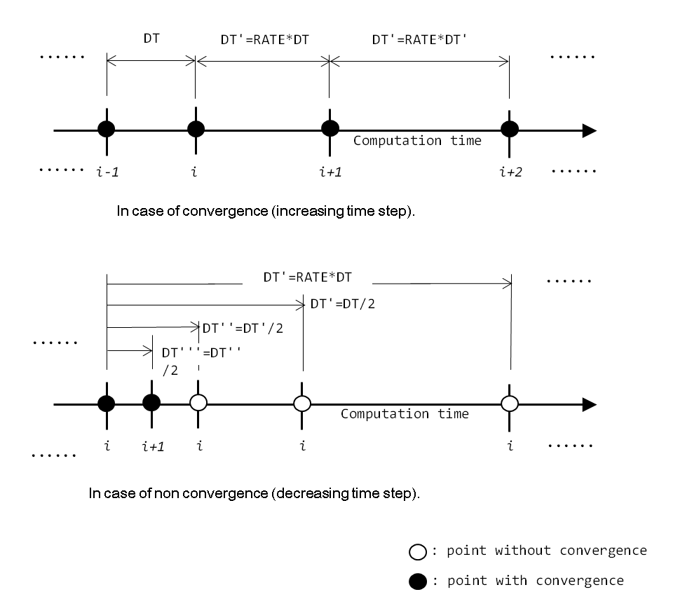
When automatic time step is set up (
automatic = ON), the simulator calculate and update the time step internally depending on the convergence determination. Convergence determination of the numerical solution is governed by parameters in the deck#control: (a) the residual norm of the linear solverconvergence-tolerance-valuein#linear-solver, (b) the residual normnl-toleranceof the non-linear iterative calculation in#primary-variable. When the two convergence criterions are not satisfied, the numerical solution of the current step is said not converged and the time step size is divided by 2. Note that using the convergence mitigation optionstimestep-convergenceallows to relax the convergence determination of condition (a) above by accepting convergence if the decrease of the residual norm is lower than thetimestep-convergencevalue (even if it is higher than theconvergence-tolerance-valuevalue).When fixed time step is set up (
automaticcard set toOFF), the time steps should be fixed with the table entryDTIM. In this case, the computation will continue until the total number of steps is reached whatever the convergence situation of the numerical solution.
See also
#control>linear-solver,
#control>nonlinear-solver,
#condition>initial
Example
Example 1: Automatic time step mode
#timestep
   automatic = ON
   time-unit = DAY       ! YEAR, WEEK, DAY, HOUR, MINUTE, SECOND
   start-time = 0.0
   end-time = 1.E30
   ndt = 100000
   dt0 = 1.E-2
   dtmax = 1.E20
   rate = 1.20
   timestep-convergence = 0.0
   *table
       primary-variable  timestep-tolerance
       PG                1.0E-06
       SW                1.0E-06
#end-of-timestep
Example 2: Manual time step mode
#timestep
   automatic = OFF
   time-unit = DAY ! YEAR, WEEK, DAY, HOUR, MINUTE, SECOND
   start-time = 0.0
   ndt = 100000
   *table |manual-timestep|
       ntim  dtim
       10    1.E-3
       30    3.E-3
       50    5.E-3
       80    1.E-2
       1000  3.E-2
#end-of-timestep
Flow-type
Description
GETFLOWS is capable to model two types of flow: Manning-type overland flow and Darcy-type underground fluid flow. This card defines the flow type to be used in each grid cell.
Identifier
| Starting deck | #flow-type |
| Ending deck | #end-of-flow-type |
List of cards
| Card name | Type | Description | Default |
|---|---|---|---|
| FLOW-TYPE | string | Type of flow | No |
if MANNING or M
then Manning-type overland flow |
|||
if DARCY or D
then Darcy-type underground fluid flow |
The flow type (Manning or Darcy) is defined on all grids of the region. Different flow type can be defined on different regions. The syntaxes available for setting up the flow type on each sub-region are listed in the following examples.
See also
design>region, design>alias-region
Examples
Example 1: Set up by region name’s name
#flow-type
 *table
     region   flow-type
     ALL      DARCY
     Surface  MANNING
#end-of-flow-type
Example 2: Set up by grid cell number (IJK)
#flow-type
    *table
        i-min i-max j-min j-max k-min k-max flow-type
        1     14    1     12    1     1     DARCY
        1     14    1     12    2     2     MANNING
#end-of-flow-type
Example 3: Set up by region name and card name
#flow-type
      ALL.flow-type = DARCY
      Surface.flow-type = MANNING
#end-of-flow-type
Example 4: Set up by input in sequential cell order
#flow-type
   *sequence-cell
      D D D D M M M M D D D D D D D D D D D D D D D D
#end-of-flow-type
Nb-equation
Description
Set up the number of equation to be solved at each cell.
Identifier
| Starting deck | #nb-equation |
| Ending deck | #end-of-nb-equation |
List of cards
| Card name | Type | Description | Default |
|---|---|---|---|
| nb-equation | integer | Number of equation to be solved in each cell | No |
See also
None
Examples
Example 1:
#nb-equation
  *table
      i-min i-max j-min j-max k-min k-max neq
      1     3     1     2     1     4     2
    surface.neq = 2
#end-of-nb-equation
Lsm-control
Description
Set up the parmeters of the land-surface model. Note that the weather
data are specified in the #land deck.
Identifier
| Starting deck | #lsm-control |
| Ending deck | #end-of-lsm-control |
List of cards
| Card name | Type | Description | Default |
|---|---|---|---|
| surface-heat-method | string | define the heat surface computation method | No |
| if ‘approximation’, no coupling with the subsurface, the surface temperature is obtained by approximate solution method. | |||
| if ‘single-layer-model’, no coupling with the subsurface, the surface temperature is obtained by a single-layer model. | |||
| if ‘coupling’, the surface heat is defined via a coupling between the surface and the subsurface. | |||
| use-canopy-litter | string | use of tree canopy and litter tanks | No |
| if ON, consider tree canopy and litter tanks. | |||
| if OFF, do not consider tree canopy and litter tanks. | |||
| snow-cover-method | string | method to process the snow accumulation | No |
| if ‘heat-balance’, consider snow cover using heat balance method | |||
| if ‘sugawara’, consider snow cover using Sugawara’s method. | |||
| if OFF, do not consider snow cover. | |||
| solar-radiation-method | string | Input method for solar radiation | No |
| if ‘direct’, direct input of solar radiation | |||
| if ‘indirect’, input sunshine hours and latitude to calculate the solar radiation. | |||
| start-date-of-simulation | string | date of the start of the simulation (YYYY-MM-DD) | No |
| snowmelt-temperature | float | temperature (°C) to discriminate between precipitation falling as rain or snow | No |
| sugawara-parameter | float | Snowmelt parameter, used if snow-cover-method is ‘sugawara’ | No |
See also
#land>lsm-rainfall, #land>lsm-wind-speed, #land>lsm-daylight-hour, #land>lsm-relative-humidity, #land>lsm-albedo, #land>lsm-storage, #land>lsm-air-temperature
Examples
Example:
#lsm-control
    surface-heat-method = single-layer-model
    use-canopy-litter = OFF
    use-snow-cover = ON
    solar-radiation-method = indirect
    start-date-of-simulation = 2005-1-1
    snowmelt-temperature = 2.0
    sugawara-parameter = 0.0
#end-of-lsm-control
Condition
The deck #condition is used to set up the general
condition of the simulation, including the initial condition and the
parameter adjustments. The deck can have one card (‘use-hydrostatic’)
and up to seven decks (#standard, #initial,
#hydrostatic, #adjust>parameter,
#adjust>waterlevel, #adjust>cav,
#adjust>prmch).
Its identifier is as follow.
| Starting deck | #condition |
| Ending deck | #end-of-condition |
Cards
Description
The card use-hydrostatic is used to activate the
hydrostatic condition at the starting of the simulation (modification of
the initial condition).
- If
use-hydrostatic = on, the initial condition (defined in the deck#initial) will be modified to enforce hydrostatic condition defined in thehydrostaticdeck (thehydrostaticdeck is required in this case). - If
use-hydrostatic = off, the initial condition (defined in the deck#initial) will be set up without modification.
| Card name | Type | Description | Default |
|---|---|---|---|
| use-hydrostatic | string | Activate the hydrostatic condition | off |
if on then hydrostatic
condition is enforced (require the deck #hydrostatic) |
|||
if off then hydrostatic
condition is not enforced |
See also
#condition>initial, #condition>hydrostatic,
Example
#condition
   use-hydrostatic = on

   [...]
#end-of-condition
Standard
Description
Define the standard values for the pressure, temperature and gravitational acceleration at sea level on Earth.
Identifier
| Starting deck | #standard |
| Ending deck | #end-of-standard |
List of cards
| Card name | Type | Description | Default |
|---|---|---|---|
| standard-pressure | float | Standard pressure (kgf/cm2) | 1.033 |
| standard-temperature | float | Standard temperature (oC) | 15.0 |
| reference-temperature | float | Reference temperature (oC) | 15.0 |
| gravity | float | Acceleration due to gravity (m/s2) | 9.80665 |
The standard pressure is used to calculate the formation volume factor, the viscosity coefficient and the porosity. The default value of the standard pressure is 1.033kgf/cm2 and the default value of the gravitational acceleration is 9.80665m/s2.
See also
None
Example
#standard
   standard-pressure = 1.033
   gravity = 9.80665
#end-of-standard
Initial
Description
Define the initial condition (the value of the primary variables at
the starting of the simulation). If the card
use-hydrostatic of the deck #condition is set
up to on, the initial condition will be modified to enforce
the hydrostatic condition.
Identifier
| Starting deck | #initial |
| Ending deck | #end-of-initial |
List of cards
The cards available in the deck initial are the primary
variables that depends on the problem-type. The table below describe the
primary variables for the problem type 3.
| Card name | Type | Description | Default |
|---|---|---|---|
| Pg | float | Gas phase pressure (kgf/cm2) | No |
| Sw | float | Aqueous phase saturation (frac.) | No |
In this deck, the value of the primary variables such as gas pressure and water saturation should be given to all the grid cells at the start of calculation. There are two options for this configuration:
Assign an user-defined primary variable value directly to each cell. This method is suitable for continuing an computation job from an existing calculation result.
To assign some initial condition automatically following the
hydrostatic condition, see the deck #hydrostatic.
See also
Examples
Example 1: Set up by region name
#initial
    *table
        region      Pg    Sw
        Atmosphere  1.033 0.001
        Surface     1.033 0.001
        UnderGround 1.033 0.1
#end-of-initial
Example 2: Set up by the cell number
#initial
    *table
        i-min i-max j-min j-max k-min k-max Pg    Sw
        1     4     1     2     1     1     1.033 0.001
        1     4     1     2     2     2     1.033 0.001
        1     4     1     2     3     4     1.033 0.1
#end-of-initial
Example 3: Set up by the region name and card
#initial
    UnderGround.Pg = 1.10
    UnderGround.Sw = 0.50
#end-of-initial
Example 4: Set up by list cell ordering
#initial
    *import-gfbase
        <output/003/main.bin.093>
#end-of-initial
Hydrostatic
Description
The deck hydrostatic allows to set up the hydrostatic
pressure condition option (modification of the initial condition in the
entire field based on the standard aqueous surface level). This deck is
optional. It is required only if the card use-hydrostatic
of the deck #condition is set up to on.
Identifier
| Starting deck | #hydrostatic |
| Ending deck | #end-of-hydrostatic |
List of cards
| Card name | Type | Description | Default |
|---|---|---|---|
| reference-layer | string | Defines the designation mode of the standard aqueous surface level | No |
| = FWL: Designation by elevation values | |||
| integer | = |
||
| reference-point | string | Defines the origin of the standard aqueous surface level (effective only if reference-layer is defined as an integer) | grid |
| = grid: cell center | |||
| = corner: cell top surface | |||
| elevation | float | Water level from the standard aqueous surface (m) | 0.0 |
| density | float | Density of aqueous phase (g/cm3) | 1.0 |
| water-type | string | Solution condition | fresh |
| = fresh: Freshwater without solute | |||
| = saturated: Solution saturated of solute | |||
| xopt | integer | Option to select the initial values of the primary variables. This option consists in a two-digit binary number (such as 10 or 11) where the first digit corresponds to the gas pressure and the second to the aqueous saturation. If equal to “0”, the variable is not initialized, if equal to “1” the variable is initialized. | 11 |
| reference-pressure | float | Standard gas phase pressure (kgf/cm2) | 1.033 |
| reference-capillary-pressure | float | Standard capillary pressure (kgf/cm2) | 0.0 |
Generate automatically the initial values at each cell by assuming hydrostatic pressure condition in the depth direction. First, the water level is assigned, either by layer or elevation. Then, the pressure under the water level is set up as the hydrostatic pressure and the water saturation is defined as 1.0. Over the water level, the gas pressure and water saturation are assigned to the atmospheric pressure and the residual water saturation respectively.

Examples
Example 1:
#hydrostatic
*table
region reference-layer reference-point elevation density xopt reference-pressure reference-pc  water-type
all    fwt             grid            0.0       1.0     11   1.033              0.0           fresh
*table
 i-min i-max j-min j-max k-min k-max reference-layer reference-point elevation density xopt reference-pressure reference-pc water-type
 1     4     1     2     1     1     3               grid            0.0       1.0     11   1.033              0.0          fresh
 1     4     1     2     2     2     3               grid            0.0       1.0     11   1.033              0.0          fresh
 1     4     1     2     3     4     3               grid            0.0       1.0     11   1.033              0.0          fresh
#end-of-hydrostatic
Example 2: Set up by region name under the hydrostatic condition
#hydrostatic
*table
region reference-layer reference-point elevation density xopt reference-pressure reference-pc
all    3               GRID            0.0       1.0     11   1.033              0.0
#end-of-hydrostatic
Example 3: Set up by cell range under the hydrostatic condition
#hydrostatic
*table
i-min i-max j-min j-max k-min k-max reference-layer reference-point elevation density xopt reference-pressure reference-pc
1     4     1     2     1     1     3               grid            0.0       1.0     11   1.033              0.0
1     4     1     2     2     2     3               grid            0.0       1.0     11   1.033              0.0
1     4     1     2     3     4     3               grid            0.0       1.0     11   1.033              0.0
#end-of-hydrostatic
Flow-velocity-field
[description coming later]
Example:
#flow-velocity-field
  velocity-field = steady
  binary-file = <output/003/main.bin.093>
#end-of-flow-velocity-field
Adjust>parameter
The decks present in #adjust are used to force the
fluctuation of some variables with time during the simulation. Water
level externl force is set up in the #adjust-waterlevel
deck. The other supported parameters are set up in the
#adjust-parameter deck. Note that the gfbase
format for adjustment (cav file and prmch
file) can still be used instead of the gfcard format (see
below).
Description
Define the fluctuation of some variables (pressure, saturation, absolute permeability, etc) due to external force, excavation, etc.
Identifier
| Starting deck | #adjust-parameter |
| Ending deck | #end-of-adjust-parameter |
List of cards
| Card name | Type | Description | Default |
|---|---|---|---|
| time-unit | string | Time unit | DAY |
if year then Year |
|||
if day then Day |
|||
if hour then Hour |
|||
if minute then Minute |
|||
if second then Second |
|||
| start-time | float | Starting time of primary variable fluctuation | No |
| end-time | float | The ending time of primary variable fluctuation | No |
| primary-variable | string | The primary variable to change | No |
| PG: Vapor phase pressure (kgf/cm2) | |||
| SW: Aqueous phase saturation (frac.) | |||
| SG: Vapor phase saturation (frac.) | |||
| RS 1, RS2: Solute concentration in the aqueous phase (m3/m3) | |||
| RG1: Solute concentration in the gas phase (m3/m3) | |||
| TF: The temperature of fluid phase (oC) | |||
| TS: The temperature of solid phase (oC) | |||
| start-value | float | The value of primary variable at the start time | No |
| end-value | float | The value of primary variable at the ending time | No |
| time-unit | string | Time unit, (YEAR: Year, DAY: Day, HOUR: Hour, MIN: Minute, SEC: Second) | DAY |
| time | float | Starting time of property change | No |
| effective-porosity | float | Effective porosity | No |
| abs-perm | float | Absolute permeability (mD) | No |
| abs-perm-i- | float | Absolute permeability at the I-side of the cells (mD) | No |
| abs-perm-i+ | float | Absolute permeability at the I+side (mD) | No |
| abs-perm-j- | float | Absolute permeability at the J-side (mD) | No |
| abs-perm-j+ | float | Absolute permeability at the J+side (mD) | No |
| abs-perm-k- | float | Absolute permeability at the K-side (mD) | No |
| abs-perm-k+ | float | Absolute permeability at the K+side (mD) | No |
| abs-perm-in | float | Absolute permeability in the specified range (mD) | No |
| abs-perm-in-i- | float | Absolute permeability in the I-direction of specified range (mD) | No |
| abs-perm-in-j- | float | Absolute permeability in the J-direction of specified range (mD) | No |
| abs-perm-in-k- | float | Absolute permeability in the K-direction of specified range (mD) | No |
| abs-perm-interior | float | Absolute permeability of the inner boundary of the specified range boundary (mD) | No |
| abs-perm-interior-i- | float | Absolute permeability located medial (I-side) to specified range boundary (mD) | No |
| abs-perm-interior-i+ | float | Absolute permeability located medial (I+side) to specified range boundary (mD) | No |
| abs-perm-interior-j- | float | Absolute permeability located medial (J-side) to specified range boundary (mD) | No |
| abs-perm-interior-j+ | float | Absolute permeability located medial (J+side) to specified range boundary (mD) | No |
| abs-perm-interior-k- | float | Absolute permeability located medial (K-side) to specified range boundary (mD) | No |
| abs-perm-interior-k+ | float | Absolute permeability located medial (K+side) to specified range boundary (mD) | No |
| abs-perm-out | float | Absolute permeability located lateral to specified range boundary (mD) | No |
| abs-perm-out-i- | float | Absolute permeability located lateral (I-side) to specified range boundary (mD) | No |
| abs-perm-out-i+ | float | Absolute permeability located lateral (I+side) to specified range boundary (mD) | No |
| abs-perm-out-j- | float | Absolute permeability located lateral (J-side) to specified range boundary (mD) | No |
| abs-perm-out-j+ | float | Absolute permeability located lateral (J-side) to specified range boundary (mD) | No |
| abs-perm-out-k- | float | Absolute permeability located lateral (K-side) to specified range boundary (mD) | No |
| abs-perm-out-k+ | float | Absolute permeability located lateral (K+side) to specified range boundary (mD) | No |
| manning | float | Equivalent roughness coefficient (m-1/3s) | No |
| manning-i- | float | Equivalent roughness coefficient at the I-side (m-1/3s) | No |
| manning-i+ | float | Equivalent roughness coefficient at the I+side (m-1/3s) | No |
| manning-j- | float | Equivalent roughness coefficient at the J-side (m-1/3s) | No |
| manning-j+ | float | Equivalent roughness coefficient at the J+side (m-1/3s) | No |
| compressibility | float | Solid compressibility (1/kgf/cm2) | No |
| water-xir | float | Residual saturation of the aqueous phase | No |
| gas-xir | float | Residual saturation of the gas phase | No |
| napl-xir | float | Residual saturation of the NAPL phase | No |
| lg-capillary-pressure | string | Table name of capillary pressure between liquid and gas phases | No |
| lg-kr-table s | tring T | able name of relative permeability between liquid and gas phases N | o |
| lg-kr-table-horizontal | string | Table name of relative permeability on horizontal plane between liquid and gas phase | No |
| lg-kr-table-up | string | Table name of upper surface relative permeability between liquid and gas phase | No |
| lg-kr-table-down | string | Table name of upper surface relative permeability between liquid and gas phases | No |
| wn-pc-table | string | Table name of capillary pressure between aqueous and NAPL phases | No |
| wn-kr-table | string | Table name of relative permeability between aqueous and NAPL phases | No |
| wn-kr-table-horizontal | string | Table name of relative permeability on horizontal surface between aqueous and NAPL phases | No |
| wn-kr-table-up | string | Table name of upper surface relative permeability between aqueous and NAPL phases | No |
| wn-kr-table-down | string | Table name of undersurface relative permeability between aqueous and NAPL phases | No |
In this deck, primary variables and geological properties time-varying fluctuations are assigned to assigned to any grid cells. Assignable primary variables depend on the fluid system. In the case of the water-gas two-phase flow analysis, the saturation of vapor phase pressure and aqueous phase is explicitly given. Linearly-interpolated values are used for the aqueous surface level at the arbitrary time between starting time and ending time.
Note that the end-time value should be greater than the
start-time value. Also, all time range that overpass the
global computation time range specified in the #timestep
deck are discard.
The time varying geological properties should be given to arbitrary grid cells.
This configuration is effective only when the calculation time point has passed the defined start time (card TIME).
Regarding solid properties, the parameters that can be adjusted are
the effective porosity, absolute permeability, Manning’s roughness
coefficient, compressibility, residual saturation ratio, capillary
pressure, and relative permeability. For the capillary pressure and the
relative permeability, the tables that control them can be adjusted,
tables defined in multiphase>define-correlation deck. In
the case of adjustment to the cell group within the arbitrary area of
sequence cell numbers, the absolute permeability is assigned to the
medial side of the specified range. When one want to model the
excavation of a ground-based open channel or a rock underground tunnel,
the loose area can be accounted for and the amount of fluid passing the
slope after the excavation can be controlled.

See also
#effective-porosity,
#absolute-permeability,
#manning-coefficient, #compressibility, #multiphase>define-correlation,
#multiphase>assign-correlation,
#irreducible-saturation
Examples
Example 1: Set up by region name
#adjust-parameter
    *table
        time-unit start-time end-time region    primary-variable start-value end-value
        DAY       0.0        10.0     UpStream  PG               1.01        1.02
        DAY       10.0       20.0     UpStream  PG               1.02        1.03
        DAY       20.0       30.0     UpStream  PG               1.03        1.04
#end-of-adjust-parameter
Example 2: Set up by cell range
#adjust-parameter
    *table
        time-unit start-time end-time i-min i-max j-min j-max k-min k-max primary-variable start-value end-value
        DAY       0.0        1.E2     1     6     1     1     3     4     PG               1.0         5.0
#end-of-adjust-parameter
Example 3: Set up by region name
#adjust-parameter
    *table
        time-unit time region effective-porosity abs-perm      abs-perm-i- abs-perm-i+ abs-perm-j- abs-perm-j+ abs-perm-k- abs-perm-k+
        DAY       0.0  ALL    0.2                10.           100.             100.             100.             100.             100.             100.
#end-of-adjust-parameter
Example 4: Set up by cell range
#adjust-parameter
    *table
        time-unit, time, i-min, i-max, j-min, j-max, k-min, k-max, water-xir, gas-xir
        DAY 0.0 1   6  1 10 3   4   0.001  0.0
#end-of-adjust-parameter
Adjust>waterlevel
Description
Define the water level fluctuation external force.
Identifier
| Starting deck | #adjust-waterlevel |
| Ending deck | #end-of-adjust-waterlevel |
List of cards
| Card name | Type | Description | Default |
|---|---|---|---|
| time-unit | string | Time unit | DAY |
if year then Year |
|||
if day then Day |
|||
if hour then Hour |
|||
if minute then Minute |
|||
if second then Second |
|||
| start-time | float | Starting time of water level fluctuation external force | No |
| end-time | float | Ending time of water level fluctuation external force | No |
| water-type | float | Solution condition | FRESH |
| = FRESH: Freshwater without solute | |||
| = SATURATED: Saturated solution of the solute | |||
| start-value | float | Water level at the start time (m) | No |
| end-value | float | Water level at the ending time (m) | No |
This deck control the adjustment of the time-varying dynamic boundary
condition of water level at any grid cells. Main usage of waterlevel
adjustemnt deck is to model the water level fluctuation of lakes or
oceans area. Aqueous surface level at any time between
start-time and end-time are computed by linear
interpolation. Note that the latter must be greater than the former.
Also, all time range that overpass the global computation time range
specified in the #timestep deck are discard.
See also
None
Examples
Example 1: Set up by region name
#adjust-waterlevel
    *table
        time-unit start-time end-time region     start-value end-value
        DAY       0.0        1.0      UpStream   1.0         0.0
        DAY       1.0        2.0      UpStream   0.0         1.0
        DAY       2.0        3.0      UpStream   1.0         0.0
#end-of-adjust-waterlevel
Example 2: Set up by cell range
#adjust-waterlevel
    *table
        time-unit start-time end-time i-min i-max j-min j-max k-min k-max start-value end-value
        DAY       0.0        1.0      1     6     1     1     3     4     1.0         2.0
#end-of-adjust-waterlevel
Adjust: Legacy gfbase input format
Description
Define the time-varying change of the geological properties.
Identifier
| Starting deck | #cav |
| Ending deck | #end-of-cav |
| Starting deck | #prmch |
| Ending deck | #end-of-prmch |
Example
#adjust
    #cav
        *import-gfbase
            <../tests-gfbase/gfbase-files/cav.03to14.v23.KYU_SAGYO.txt>
    #end-of-cav

    #cav
        *import-gfbase
            <../tests-gfbase/gfbase-files/cav.03to14.v23.KYU_SAGYO.txt>
    #end-of-cav
#end-of-adjust
Fluid
This deck contains #properties that groups all the
settings related to the physical properties of fluid and
#pressure-volume-temperature that define the
pressure-volume-temperature table, that is the function of some fluid
properties with the pressure.
Properties
Define the physical properties of each fluid (water, gas, napl).
List of settings in
#properties
| Card name | Type | Description | Default |
|---|---|---|---|
| normal-fvf | float | Formation volume factor defined at
condition>standard (m3/m3) |
No |
| fluid-compressibility | float | Compressibility of the fluid (1/ (kgf/cm2)) | No |
| normal-viscosity | float | Viscosity coefficient defined at
condition>standard (cP) |
No |
| viscosity-increment | float | Viscosity variation factor per pressure variation unit (1/kgf/cm2) | No |
| fluid-density | float | Density of fluid phase defined at
condition>standard (g/cm3) |
No |
| method-pvt | string | Definition method for the relationship between “pressure - formation volume factor - viscosity coefficient”. | No |
| = equation: linear formula | |||
| = table: table format |
In this deck, the different physical properties of each fluid can be simultaneously input. Fluid names are fixed depending on the type of simulation (water, gas, etc)
See also
#object>#[fluid]
Example
Example 1: Set up by table
#properties
    *table
        fluid-phase normal-fvf compressibility normal-viscosity viscosity-increment density method-pvt
        water       1.0        1.e-5           1.e0             1.e-5               1.0     equation
        gas         1.0        1.e-5           0.0182           1.e-5               1.22e-5 equation
        napl        1.0        1.e-5           1.e0             1.e-5               1.0     value
#end-of-properties
Example 2: Set up by fluid phase name and card’s name
#properties
    water.normal-fvf = 1.E0
    water.compressibility = 1.E-5
    water.normal-viscosity = 1.E0
    water.viscosity-increment = 1.E-5
    water.density = 1.E0
    water.method-pvt = equation
    gas.method-pvt = value
#end-of-properties
Example 3: Set up by object (no yet supported)
#properties
    water = [&my_groundwater]
    gas = [&air]
    water.density = [&air.density]
#end-of-properties
Normal-fvf
Define the formation volume factor at standard pressure condition. No
default value for the volume factor has to be defined for each fluid
phase. The standard pressure is defined using the deck
condition>standard. Fluid names are fixed depending on
the type of simulation or registered in a fluid object.
Compressibility
Define the compression ratio of the fluid phase. No default value for the compression ratio must be defined for each fluid phase. Fluid names are fixed depending on the type of simulation or registered in a fluid object.
normal-viscosity
Define the viscosity value at standard conditions of pressure and
temperature. No default value for the viscosity coefficient must be
defined for each target fluid phase. The standard pressure is defined in
the condition>standard deck. Fluid names are fixed
depending on the type of simulation or registered in a fluid object.
Viscosity-increment
Define the viscosity variation factor per pressure variation unit. No
default value for the viscosity variation factor is defined; the factor
must be defined for each fluid phase. The standard pressure is defined
in the condition>standard deck. Fluid phase names used
herein must be defined in the control>job>fluid deck
or registered in a fluid object.
Density
Define the fluid density at standard pressure. No default value for
the density of the fluid phase is defined; the value must be defined for
each fluid phase. The standard pressure is defined in the
condition>standard deck. Fluid names are fixed depending
on the type of simulation or registered in a fluid object.
Method-pvt
Define the relationship between the pressure, the formation volume
factor and the viscosity. When using the equation format input, the
aqueous phase, the formation volume factor of the NAPL liquid phase and
the viscosity is evaluated by the sum of the change for each unit of
volume and pressure changes in various state standards. This variation
is defined in the #fluid>#properties table under the
compressibility column and in the
#viscosity-increment deck. The volume of gas-phase
coefficients is evaluated in a manner inversely proportional to
pressure. When using the table format input, the relation is set up with
values entered as a table in the
pressure-volume-temperature deck. No default input format
is set up; also the input format must be defined for each fluid phase
present in the analysis. Fluid names are defined automatically from the
problem type.
Pressure volume temperature
Description
Define the relationship between the pressure, the formation volume factor and the viscosity of each phase in the table format.
Identifier
| Starting deck | #pressure-volume-temperature |
| Ending deck | #end-of-pressure-volume-temperature |
List of cards
| Specified item | Type | Description | Default |
|---|---|---|---|
| pressure | float | Pressure (kgf/cm2) | No |
| water-fvf | float | Formation volume factor of the aqueous phase (m3/m3) | No |
| gas-fvf | float | Formation volume factor of the gas phase (m3/m3) | No |
| water-viscosity | float | Viscosity of the aqueous phase (cP) | No |
| gas-viscosity | float | Viscosity of the gas phase (cP) | No |
For each fluid phase, the card method-pvt card of the
fluid>properties deck must be set up to
method-pvt=value. The pressure set up in the table must be
included in the range min-value, max-value defined in the
#solver deck. Fluid names are fixed depending on the type
of simulation or registered in a fluid object.
See also
#control>linear-solver,
#control>nonlinear-solver,
#method-pvt, #fluid>properties,
[#object>#[fluid]]
Example
#pressure-volume-temperature
    *table
        pressure water-fvf  gas-fvf   water-viscosity gas-viscosity
        -1000.   1.0        1.0       1.0             0.0182
        0.000    1.0        1.0       1.0             0.0182
        1.033    1.0        1.0       1.0             0.0182
        2.000    0.9999573  0.5       1.0             0.0182
        5.000    0.2        1.0       0.9998249       0.0182
        10.00    0.1        1.0       0.9996042       0.0182
        20.00    0.9991628  0.05      1.0             0.0182
        30.00    0.033      0.9987214 1.0             0.0182
        40.00    0.025      0.9982800 1.0             0.0182
        50.00    0.9978386  0.02      1.0             0.0182
        100.0    0.9956316  0.01      1.0             0.0182
        500.0    0.002      0.9956316 1.0             0.0182
        1000.    .9956316   0.001     1.0             0.0182
#end-of-pressure-volume-temperature
Solid
Effective-porosity
Description
Define the effective porosity at standard pressure.
Identifier
| Starting deck | #effective-porosity |
| Ending deck | #end-of-effective-porosity |
List of cards
| Card name | Type | Description | Default |
|---|---|---|---|
| effective-porosity | float | Effective porosity (-) | No |
The effective porosity at standard pressure should be defined for the
entire grid. The standard pressure is defined in
condition>standard deck.
The effective porosity setting can be used to freeze the value of the
primary variables such as pressure and saturation for particular cells.
When a large value of effective porosity is defined (effective-porosity
\(\geq\) 1E10), and in case of setting
“exclude-cell=ON” in the #solver deck, the cells with
effective porosity greater than 1E10 are excluded from the computation
by the solver.
See also
#control>linear-solver,
#control>nonlinear-solver,
#solid, #store>object>#[solid]
Examples
Example 1: Set up by region name
#effective-porosity
    *table
        region      effective-porosity
        Atmosphere  1.0E30
        Surface     1.0E30
        Imperm      1.0E30
        UnderGround 0.4E0
        UpStream    1.0E30
#end-of-effective-porosity
Example 2: Set up by cell range
#effective-porosity
*table
    i-min i-max j-min j-max k-min k-max effective-porosity
    1     4     1     2     1     1     1.E30
    1     4     1     2     2     2     1.E0
#end-of-effective-porosity
Example 3: Set up by region name and card name
#effective-porosity
    Atmosphere.effective-porosity = 1.0E30
    UnderGround.effective-porosity = 0.4
#end-of-effective-porosity
Example 4: Set up by input in sequential cell order
#effective-porosity
    *sequence-cell
        1.e30 1.0 0.3 0.3 0.3 0.3 0.3 0.3 0.3 0.3 0.3 0.3
#end-of-effective-porosity
Absolute-permeability
Description
Define the absolute permeability.
Identifier
| Starting deck | #absolute-permeability |
| Ending deck | #end-of-absolute-permeability |
List of cards
| Card name | Type | Description | Default |
|---|---|---|---|
| file-import-cell-or-side | string | side or cell:
type of content of the file imported with *import-gfbase, (
when the file is binary or a sequence of values) |
No |
| abs-perm | float | Absolute permeability of the cell (mD) | No |
| abs-perm-i- | float | Absolute permeability at the I-side of the cell (mD) | No |
| abs-perm-i+ | float | Absolute permeability at the I+side of the cell (mD) | No |
| abs-perm-j- | float | Absolute permeability at the J-side of the cell (mD) | No |
| abs-perm-j+ | float | Absolute permeability at the J+side of the cell (mD) | No |
| abs-perm-k- | float | Absolute permeability at the K-side of the cell (mD) | No |
| abs-perm-k+ | float | Absolute permeability at the K+side of the cell (mD) | No |
The absolute permeability should be defined for the entire grid. The
method of inputting the absolute permeability for isotropic media is
different from the method for anisotropic media. In the case of
isotropic media, only the value of a whole cell is necessary
(abs-perm). In the case of anisotropic media, the absolute
permeability should be defined for each cell side (abs-perm-i-, …). The
isotropic media is equivalent to the anisotropic media with the same
value of absolute permeability for each cell side. Note that the
relative permeability setting of deck #define-correlation
can also be used to define an anisotropic media.
See also
#solid, #store>object>#[solid], #define-correlation
Examples
Example 1: Set up by region name
#absolute-permeability
   *table
       region      abs-perm-i- abs-perm-i+ abs-perm-j- abs-perm-j+ abs-perm-k- abs-perm-k+
       Atmosphere  1.E10       1.E10       1.E10       1.E10       1.E10       1.E10
       Surface     1.E10       1.E10       1.E10       1.E10       1.E10       1.E10
       Imperm      0.E0        0.E0        0.E0        0.E0        0.E0        0.E0
       UnderGround 1.E3        1.E3        1.E3        1.E3        1.E3        1.E3
       UpStream    1.E10       1.E10       1.E10       1.E10       1.E10       1.E10
       DownStream  1.E10       1.E10       1.E10       1.E10       1.E10       1.E10
#end-of-absolute-permeability
Example 2: Set up by cell range
#absolute-permeability
   *table
       i-min  i-max  j-min  j-max  k-min  k-max  abs-perm
       1      4      1      2      4     4       1.E3
#end-of-absolute-permeability
Example 3: Set up by region name and card name
#absolute-permeability
    UpStream.abs-perm-i-= 1.E10
    UpStream.abs-perm-i+= 1.E10
    UpStream.abs-perm-j-= 1.E10
    UpStream.abs-perm-j+= 1.E10
    UpStream.abs-perm-k-= 1.E10
    UpStream.abs-perm-k+= 1.E10
    DownStream.abs-perm = 1.E10
#end-of-absolute-permeability
Example 4: Set up by input in sequential cell order
In sequential input mode, the absolute permeability values of the six sides of each cell should be given. Therefore, the number of values to be given is 6 times the number of cells. The order is (with the cell numbered starting from increasing index I, then J, then K):
abs-perm-i- abs-perm-i+ abs-perm-j- abs-perm-j+ abs-perm-k- abs-perm-k+
abs-perm-i- abs-perm-i+ abs-perm-j- abs-perm-j+ abs-perm-k- abs-perm-k+
...
#absolute-permeability
*sequence-cell
1.E10 1.E10 1.E3 1.E3 1.E3 1.E3 1.E3 1.E3 1.E3 1.E3 0.E0
#end-of-absolute-permeabilityExample 5: Set up by external binary file
Here, the user has to set up the card
file-import-cell-or-side to cell or
side in order to specify if the binary file contains one
value per cell or one value per side.
#absolute-permeability
   file-import-cell-or-side = 'cell'
   *import-gfbase
      <abs-perm.bin>
#end-of-absolute-permeability
Example 6: Set up by external sequence file
Here, the user has to set up the card
file-import-cell-or-side to cell or
side in order to specify if the file contains one value per
cell or one value per side.
#absolute-permeability
   file-import-cell-or-side = 'side'
   *import-gfbase
      <abs-perm-sequence.txt>
#end-of-absolute-permeability
Absolute-permeability-factor
Description
Define the coefficient that multiply the absolute permeability to take into account the variation of absolute permeability depending on the fluid phase. This is used for instance to model the slip effect of gas molecule (Klinkenberg 1941).
Identifier
| Starting deck | #abs-perm-factor |
| Ending deck | #end-of-abs-perm-factor |
List of cards
| Card name | Type | Description | Default |
|---|---|---|---|
| abs-perm-factor-water | float | Multiplication factor of the absolute permeability for the aqueous phase (-) | 1.0 |
| abs-perm-factor-gas | float | Multiplication factor of the absolute permeability for the gas phase (-) | 1.0 |
The multiplication of absolute permeability at each phase should be
defined for the entire grid. In the actual calculation, the absolute
permeability defined in #absolute-permeability deck is
multiplied by the defined scale factor value.
See also
#absolute-permeability,
#solid, #store>object>#[solid]
Examples
Example 1: Set up by region name
#abs-perm-factor
    *table
        region      abs-perm-factor-water abs-perm-factor-gas
        Atmosphere  1.0                   1.0
        Surface     1.0                   1.0
        Imperm      1.0                   1.0
        UnderGround 1.0                   2.0
        UpStream    1.0                   1.0
#end-of-abs-perm-factor
Example 2: Set up by cell range
#abs-perm-factor
    *table
        I-MIN I-MAX J-MIN J-MAX K-MIN K-MAX abs-perm-factor-water abs-perm-factor-gas
        1     4     1     2     1     1     1.0                   1.0
        1     4     1     2     2     2     1.0                   1.0
        1     4     1     2     3     4     1.0                   2.0
#end-of-abs-perm-factor
Example 3: Set up by region name and card name
#abs-perm-factor
        UnderGround.abs-perm-factor-gas = 2.0
#end-of-abs-perm-factor
Example 4: Set up by input in sequential cell order
#abs-perm-factor
    *sequence-cell
        1.0 1.0 1.0 1.0 1.0 1.0 1.0 1.0 1.0 1.0 1.0 1.0
        1.0 1.0 2.0 2.0 2.0 2.0 2.0 2.0 2.0 2.0 2.0 2.0
#end-of-abs-perm-factor
Manning-coefficient
Description
Define the Manning’s roughness coefficient for each overland flow cell of the grid.
Identifier
| Starting deck | #manning-coefficient |
| Ending deck | #end-of-manning-coefficient |
List of cards
| Card name | Type | Description | Default |
|---|---|---|---|
| surface-water-model | string | Approximate option of the overland flow | LINEARIZED-DIFFUSION-WAVE |
| manning | float | Manning’s roughness coefficient of the cell (m -1/3s) | No |
| manning-i- | float | Manning’s roughness coefficient at the I-side of the cells (m-1/3s) | No |
| manning-i+ | float | Manning’s roughness coefficient at the I+side of the cells (m-1/3s) | No |
| manning-j- | float | Manning’s roughness coefficient at the J-side of the cells (m-1/3s) | No |
| manning-j+ | float | Manning’s roughness coefficient at the J+side of the cells (m-1/3s) | No |
This deck defines the Manning’s roughness coefficient of overland
flow cells of the grid when Manning type of flow is specified in the
#flow-type deck. Different Manning’s roughness coefficient
for each direction can be considered (isotropic media or anisotropic
media). In the case of isotropic media, only the coefficient of a whole
cell is necessary (MANN). In the case of anisotropic media, the
Manning’s roughness coefficient should be defined for each cell side
(I-MANN, …).
See also
#flow-type, #solid, #store>object>#[solid]
Examples
Example 1: Set up by region name
#manning-coefficient
   surface-water-model = linearized-diffusion-wave
   *table
       region      manning-i- manning-i+ manning-j- manning-j+
       Atmosphere  n.a.       n.a.       n.a.       n.a.
       Surface     1.E10      1.E10      1.E10      1.E10
       Imperm      n.a.       n.a.       n.a.       n.a.
       UnderGround n.a.       n.a.       n.a.       n.a.
       UpStream    n.a.       n.a.       n.a.       n.a.
       DownStream  n.a.       n.a.       n.a.       n.a.
#end-of-manning-coefficient
Example 2: Set up by cell range
#manning-coefficient
   surface-water-model = linearized-diffusion-wave
   *table
       i-min i-max j-min j-max k-min k-max mann
       1     4     1     2     2     2     1.E10
#end-of-manning-coefficient
Example 3: Set up by region name and card name
#manning-coefficient
   surface-water-model = linearized-diffusion-wave
   Surface.manning = 1.e10
   Surface.manning-i- = 1.e10
   Surface.manning-i+ = 1.e10
   Surface.manning-j- = 1.e10
   Surface.manning-j+ = 1.e10
#end-of-manning-coefficient
Example 4: Set up by input in sequential cell order
#manning-coefficient
   surface-water-model = linearized-diffusion-wave
   *sequence-cell
      1.E10 0.03 0.03 0.6 0.1 2.0 1.E10
#end-of-manning-coefficient
Compressibility
Description
Define the solid phase compressibility.
Identifier
| Starting deck | #compressibility |
| Ending deck | #end-of-compressibility |
List of cards
| Card name | Type | Description | Default |
|---|---|---|---|
| compressibility | float | Solid phase compressibility (1/ (kgf/cm2)) | No |
See also
Examples
Example 1: Set up by region name
#compressibility
    *table
        region      compressibility
        Atmosphere  1.E-5
        Surface     1.E-5
        Imperm      1.E-5
        UnderGround 1.E-5
        UpSream     1.E-5
        DownStream  1.E-5
#end-of-compressibility
Example 2: Set up by cell range
#compressibility
    *table
        i-min i-max j-min j-max k-min k-max compressibility
        1     4     1     2     3     4     1.E-5
#end-of-compressibility
Example 3: Set up by region name and card name
#compressibility
    UnderGround.compressibility = 1.E-5
#end-of-compressibility
Example 4: Set up by input in sequential cell order
#compressibility
    *sequence-cell
        0.E0 0.E0 1.E-5 1.E-5 1.E-5 1.E-5 1.E-5 1.E-5 1.E-5 1.E-5
#end-of-compressibility
Irreducible-saturation
Description
Define the residual saturation ratio of the fluid phase.
Identifier
| Starting deck | #irreducible-saturation |
| Ending deck | #end-of-irreducible-saturation |
List of cards
| Card name | Type | Description | Default |
|---|---|---|---|
| water-xir | float | Residual saturation of the aqueous phase | No |
| gas-xir | float | Residual saturation of the gas phase | No |
| napl-xir | float | Residual saturation of the NAPL phase | No |
The residual saturation of each phase should be defined for all the
grid cells. Also it needs to be consistent with the residual saturation
used to create the table data of relative permeability curve assigned in
the #assign-correlation deck.
See also
#define-correlation,
#assign-correlation, #solid, store>object>#[solid]
Examples
Example 1: Set up by region name
#irreducible-saturation
   *table
       region        water-xir gas-xir
       Atmosphere    0.001     0.0
       Surface       0.001     0.0
       Imperm        0.1       0.0
       UnderGround   0.1       0.0
       UpStream      0.1       0.0
       DownStream    0.1       0.0
#end-of-irreducible-saturation
Example 2: Set up by cell range
#irreducible-saturation
   *table
       i-min i-max j-min j-max k-min k-max water-xir gas-xir
       1     4     1     2     1     2     0.001     0.0
#end-of-irreducible-saturation
Example 3: Set up by region name and card name
#irreducible-saturation
      UpStream.water-xir = 0.1
      UpStream.gas-xir   = 0.0
#end-of-irreducible-saturation
Example 4: Set up by input in sequential cell order
#irreducible-saturation
   *sequence-cell
      0.001 0.001 0.1 0.1 0.1 0.1 0.1 0.1 0.1 0.1 0.1
      0.0   0.0   0.0 0.0 0.0 0.0 0.0 0.0 0.0 0.0 0.0
#end-of-irreducible-saturation
Bulk constant
Description
Define the bulk constant (4 parameters).
Identifier
| Starting deck | #bulk-constant |
| Ending deck | #end-of-bulk-constant |
List of cards
None
See also
Examples
Example 1: Set up by region name
#bulk-constant
    *table
        region      bulk1 bulk2 bulk3 bulk4
        Atmosphere  1.E0  1.E0  1.E0  1.E0
        Surface     1.E0  1.E0  1.E0  1.E0
        Imperm      1.E0  1.E0  1.E0  1.E0
        UnderGround 1.E0  1.E0  1.E0  1.E0
        UpSream     1.E0  1.E0  1.E0  1.E0
        DownStream  1.E0  1.E0  1.E0  1.E0
#end-of-bulk-constant
Multiphase
The multiphase deck accepts the card equation as shown
in Table 12.1.
| Card name | Type | Description | Default |
|---|---|---|---|
| kr-method | string | Method of calculation of the relative permeability in multi-phase flow | No |
| Stone-1: The Stone first method | |||
| Stone-2: The Stone second method | |||
| Baker: saturation weighted interpolating method |
Define-correlation
Description
Define the multiphase flow parameters: capillary pressure and relative permeability as functions of the water content.
Identifier
| Starting deck | #define-correlation |
| Ending deck | #end-of-define-correlation |
List of cards
| Card name | Type | Description | Default |
|---|---|---|---|
| Sw | float | Saturation of wetting phase saturation | No |
| pc-water | float | Capillary pressure of water phase (kgf/cm2) | No |
| pc-gas | float | Capillary pressure of gas phase (kgf/cm2) | No |
| pc-napl | float | Capillary pressure of NAPL phase (kgf/cm2) | No |
| kr-water | float | Wetting phase relative permeability (isotropic) | No |
| kr-napl | float | Non-wetting phase relative permeability (isotropic) | No |
| kr-water-horizontal | float | Wetting phase relative permeability (horizontal component) | No |
| kr-napl-horizontal | float | Non-wetting phase relative permeability (horizontal component) | No |
| kr-water-up | float | Wetting phase relative permeability (upper component) | No |
| kr-napl-up | float | Non-wetting phase relative permeability (upper component) | No |
| kr-water-down | float | Wetting phase relative permeability (lower component) | No |
| kr-napl-down | float | Non-wetting phase relative permeability (lower component) | No |
In this data deck, the relationship between wetting phase saturation
and capillary pressure, also wetting phase saturation and relative
permeability are input in table format. Depending on the option
DIRECTION, the cards available for the table differ (see the examples
below). Linear interpolations of the discrete values given in the table
are used to estimate the intermediate values at arbitrary wetting phase
saturation during the computation. This data deck only records the table
data. Assignation of the data to the grid cells is done in
#assign-correlation deck.
See also
#solid, #assign-correlation, store>object>#[solid]
Examples
Example 1: Input of isotropic capillary pressure and relative permeability
#define-correlation
   *table |No.1-WG|
        Sw         pc-water  kr-water kr-napl
        -1.000     0.052     0.000    1.000
        0.110      0.052     0.001    0.978
        0.200      0.032     0.005    0.780
        0.300      0.027     0.009    0.575
        0.400      0.024     0.029    0.395
        0.500      0.022     0.068    0.248
        0.600      0.020     0.135    0.137
        0.700      0.018     0.239    0.062
        0.800      0.017     0.393    0.020
        0.900      0.014     0.619    0.003
        1.000      0.000     1.000    0.000
        2.000      0.000     1.000    0.000
   *import
        <multiphase_table.dat>
#end-of-define-correlation
Example 2: Input of anisotropic relative permeability
#define-correlation
   *table |No.1-WG|
       saturation pc-water kr-water-horizontal kr-napl-horizontal kr-water-up kr-napl-up kr-water-down kr-napl-down
       -1.0       0.0      0.0                 1.0                0.0         1.0        0.0           1.0
       0.001      0.0      0.0                 1.0                0.0         1.0        0.0           1.0
       0.1        0.0      0.005               0.6                0.005       0.6        0.005         1.0
       0.2        0.0      0.02                0.4                0.02        0.4        0.02          0.4
       0.3        0.0      0.04                0.28               0.04        0.28       0.04          0.28
       0.4        0.0      0.08                0.19               0.08        0.19       0.08          0.19
       0.5        0.0      0.12                0.12               0.12        0.12       0.12          0.12
       0.6        0.0      0.19                0.08               0.19        0.08       0.19          0.08
       0.7        0.0      0.28                0.04               0.28        0.04       0.28          0.04
       0.8        0.0      0.4                 0.02               0.4         0.02       0.4           0.02
       0.9        0.0      0.6                 0.005              0.6         0.005      0.6           0.005
       1.0        0.0      1.0                 0.0                1.0         0.0        1.0           0.0
       2.0        0.0      1.0                 0.0                1.0         0.0        1.0           0.0
#end-of-define-correlation
Assign-correlation
Description
Assign the table data of capillary pressure and relative permeability to the grid cells.
Identifier
| Starting deck | #assign-correlation |
| Ending deck | #end-of-assign-correlation |
List of cards
| Card name | Type | Description | Default |
|---|---|---|---|
| lg-pc-table | string | Table name of the capillary pressure between liquid phase and gas phase | No |
| lg-kr-table | string | Table name of the relative permeability between liquid phase and gas phase | No |
| lg-kr-table-horizontal | string | Table name of the relative permeability on horizontal surface between liquid phase and gas phase | No |
| lg-kr-table-up | string | Table name of the relative permeability on top surface between liquid phase and gas phase | No |
| lg-kr-table-down | string | Table name of the relative permeability on under surface between liquid phase and gas phase | No |
| wn-pc-table | string | Table name of the capillary pressure between aqueous phase and NAPL phase | No |
| wn-kr-table | string | Table name of the relative permeability between aqueous phase and NAPL phase | No |
| wn-kr-table-horizontal | string | Table name of the relative permeability on horizontal surface between aqueous phase and NAPL phase | No |
| wn-kr-up-table | string | Table name of the relative permeability on top surface between aqueous phase and NAPL phase | No |
| wn-kr-down-table | string | Table name of the relative permeability on under surface between aqueous phase and NAPL phase | No |
Note: the prefix lg and wn allows to set up
the relative permeability Kr for each fluid system. the
prefix lg- means Liquid (water only, water + NAPL) and gas
fluid system. The prefix wn- means Water and NAPL fluid
system
Note: Depending on the parameters set up, the medium is considered
isotropic or anisotropic in regard of the relative permeability. If
wn-kr-table is set up, the medium is isotropic (same value
is used for the horizontal, up and down directions). If not, the table
requires to set up the relative permeability for each direction
(horizontal, up and down).
The recorded table data of capillary pressure and relative
permeability defined in #define-correlation deck should be
assigned to all grid cells. In case of isotropic geological media, only
lg-kr-table should be assigned for the relative
permeability. In the case of anisotropic geological media, the value
should be defined for each direction of horizontal, top and under
surface.
See also
#solid, #define-correlation, store>object>#[solid]
Examples
Example 1: Set up by region name
#assign-correlation
    *table
        region       lg-pc-table  lg-kr-table
        Atmosphere   Atm-WG                       Atm-WG
        Surface      Surf-WG                      Surf-WG
        Imperm       Other-WG                     Other-WG
        UnderGround  Other-WG                     Other-WG
        UpStream     Other-WG                     Other-WG
#end-of-assign-correlation
Example 2: Set up by cell range
#assign-correlation
    *table
        i-min i-max j-min j-max k-min k-max lg-pc-table lg-kr-table-horizontal lg-kr-table-up            lg-kr-table-down
        1     4     1     2     2     2     Surf-WG                     Surf-WG                      Surf-WG              Surf-WG
#end-of-assign-correlation
Example 3: Set up by region name and card name
#assign-correlation
    Surface.lg-pc-table = Surf-WG
    Surface.lg-kr-table-table = Surf-WG
#end-of-assign-correlation
Example 4: Set up by input in sequential cell order
#assign-correlation
    *sequence-cell
        Atm-WG Surf-WG Other-WG Other-WG Other-WG Other-WG
        Atm-WG Surf-WG Other-WG Other-WG Other-WG Other-WG
#end-of-assign-correlation
Land
Rainfall
Description
Define the fluid exchange (production and injection) between the system and its environment.
Identifier
| Starting deck | #rainfall |
| Ending deck | #end-of-rainfall |
List of cards
| Card name | Type | Description | Default |
|---|---|---|---|
| time-unit | string | Time unit | DAY |
if year then Year |
|||
if day then Day |
|||
if hour then Hour |
|||
if minute then Minute |
|||
if second then Second |
|||
| start-time | float | Starting time of the fluid exchange | No |
| end-time | float | Ending time of the fluid exchange | No |
| rain-unit | string | Unit of the fluid exchange values = m3: Volume (m3/day) = mm: height of fluid per unit area (mm/day) | No |
| component | string | Component of the exchanged fluid = water or W: Water | No |
| = gas or G: Gas | |||
= (fluid_name).(solute_name):
Solute in the fluid |
|||
| = HEAT or H: Heat | |||
| rainfall | float | Volume of exchange per unit of time Positive value (FLUX>0) designs production (outflow). Negative value (FLUX<0) designs injection (inflow). | No |
| concentration | float | Concentration of solute in the fluid | No |
| temperature | float | Fluid temperature | No |
In this deck, boundary condition such as precipitation, water intake,
tail water and gas generation are assigned to any cells. The option
RAIN-UNIT="mm" is used mainly to assign the distribution of
precipitation. When this option is set up, the amount of rainfall in mm
is converted into volume in the simulator by multiplication with the
area of the projected plane of the cells. Note that the
end-time value should be greater than the
start-time value. Also, all time range that overpass the
global computation time range specified in the #timestep
deck are discard.
See also
None
Examples
Example 1: Set up by region name
#rainfall
    *table
        time-unit start-time end-time region  rain-unit component rainfall
        DAY       0.0        1.0      Surface mm        water     -0.2
        DAY       5.0        6.0      Surface mm        water     -0.3
#end-of-rainfall
Example 2: Set up by cell range
#rainfall
    *table
        time-unit start-time end-time i-min i-max j-min j-max k-min k-max rain-unit component rainfall
        DAY       0.0        1.0      1     12    1     10    2     2     mm        water     -0.2
        DAY       5.0        6.0      1     12    1     10    2     2     mm        water     -0.3
#end-of-rainfall
Evapotranspiration
Description
Define the evapotranspiration external force.
Identifier
| Starting deck | #evapotranspiation |
| Ending deck | #end-of-evapotranspiation |
List of cards
| Card name | Type | Description | Default |
|---|---|---|---|
| time-unit | string | Time unit | DAY |
if year then Year |
|||
if day then Day |
|||
if hour then Hour |
|||
if minute then Minute |
|||
if second then Second |
|||
| start-time | float | Starting time of the evapotranspiration external force | No |
| end-time | float | Ending time of the evapotranspiration external force | No |
| pet-unit | string | Unit of the evapotranspiration amount | No |
| = m3: Volume (m3/day) | |||
| = mm: Height per unit of area (mm/day) | |||
| pet | float | Amount of evapotranspiration per unit of time (> 0) | No |
In this deck, boundary condition of evapotranspiration external force
is assigned to arbitrary cells of the surface layer. When the option
pet-unit="mm" is set up, the evapotranspiration amount in
mm (PET card) is converted into volume in the simulator by
multiplication with the area of the projected plane of the cells. If the
water amount of the surface layer is lower than the evapotranspiration
amount set up by PET card, it is considered that the water of the layer
just under the surface layer can also evaporate. In this case, the
evapotranspiration efficiency table that gives the relationship between
the aqueous phase saturation of surface layer and the evaporation
efficiency should be defined (SOIL-EVAPORATION card). The table name of
evapotranspiration efficiency table should be registered in the
after-mentioned #soil-evaporation deck. Note that the
END-TIME value should be greater than the start-time value.
Also, all time range that overpass the global computation time range
specified in the #timestep deck are discard.
See also
None
soil-evaporation
Examples
Example 1: Set up by region name
#evapotranspiration
   *table
       time-unit start-time end-time region   pet-unit  pet soil-evaporation-table
       DAY       0.0        1.E30    ALL      mm        2.0 ETAB01
#end-of-evapotranspiration
Example 2: Set up by cell range
#evapotranspiration
   *table
       time-unit start-time end-time i-min i-max j-min j-max k-min k-max pet-unit  pet soil-evaporation-table
       DAY       0.0        1.E30    1     12    1     10    1     4     mm        2.0 ETAB01
#end-of-evapotranspiration
Soil-evaporation
Description
Define the evaporation efficiency table.
Identifier
| Starting deck | #soil-evaporation |
| Ending deck | #end-of-soil-evaporation |
List of cards
| Card name | Type | Description | Default |
|---|---|---|---|
| water-saturation | float | Aqueous saturation | No |
| efficiency | float | Evaporation efficiency | No |
The evaporation efficiency gives the evaporation amount according to
the water amount of surface layer. The more soil moisture there is, the
bigger evaporation amount there is. And the less soil moisture there is,
the smaller evaporation amount there is. The soil water amount
quantifies the aqueous phase saturation in the surface horizon. The
relationship between the aqueous phase saturation and the evaporation
efficiency should be input by the table format. The surface horizon
usually quantifies the geological layer just under the surface layer
(K=3). If the amount is more than the amount of evapotranspiration
defined by the #evapotranspiration, the summation of the
surface water and soil moisture at the relevant spot is the upper limit
of evapotranspiration amount.
Using an *import section, it is possible to define the
#soil-evaporation from an external file.
See also
Example
#soil-evaporation
    *table |ETAB01|
        water-saturation efficiency
        0.00             -1.00
        0.00             0.00
        0.00             0.02
        0.05             0.00
        0.00             0.08
        0.00             0.10
        0.05             0.12
        0.07             0.15
        0.09             0.18
        0.11             0.20
        0.14             0.22
        0.25             0.20
        0.30             0.28
        0.50             0.30
        0.80             0.32
        0.95             0.35
        0.99             0.38
        1.00             0.40
        1.00             0.42
        1.00             0.45
        1.00             0.48
        1.00             0.50
        1.00             1.00
    *import
        <sev.gcard>
#end-of-soil-evaporation
lsm-rainfall
Description
Define the lsm-rainfall.
Identifier
| Starting deck | #lsm-rainfall |
| Ending deck | #end-of-lsm-rainfall |
List of cards
| Card name | Type | Description | Default |
|---|---|---|---|
| time-unit | string | Time unit | DAY |
if year then Year |
|||
if day then Day |
|||
if hour then Hour |
|||
if minute then Minute |
|||
if second then Second |
|||
| start-time | float | Starting time of the fluid exchange | No |
| end-time | float | Ending time of the fluid exchange | No |
| rain-unit | string | Unit of the fluid exchange values = m3: Volume (m3/day) = mm: height of fluid per unit area (mm/day) | No |
| component | string | Component of the exchanged fluid = water or W: Water | No |
| = gas or G: Gas | |||
= (fluid_name).(solute_name):
Solute in the fluid |
|||
| = HEAT or H: Heat | |||
| rainfall | float | Volume of exchange per unit of time Positive value (FLUX>0) designs production (outflow). Negative value (FLUX<0) designs injection (inflow). | No |
| concentration | float | Concentration of solute in the fluid | No |
| temperature | float | Fluid temperature | No |
In this deck, boundary condition such as precipitation, water intake,
tail water and gas generation are assigned to any cells. The option
RAIN-UNIT=“mm” is used mainly to assign the distribution of
precipitation. When this option is set up, the amount of rainfall in mm
is converted into volume in the simulator by multiplication with the
area of the projected plane of the cells. Note that the END-TIME value
should be greater than the START-TIME value. Also, all time range that
overpass the global computation time range specified in the
#timestep deck are discard.
See also
None
Examples
Example 1: Set up by region name
#lsm-rainfall
    *table
        time-unit start-time end-time region  rain-unit component rainfall
        DAY       0.0        1.0      Surface mm        water     -0.2
        DAY       5.0        6.0      Surface mm        water     -0.3
#end-of-lsm-rainfall
Example 2: Set up by cell range
#lsm-rainfall
    *table
        time-unit start-time end-time i-min i-max j-min j-max k-min k-max rain-unit component rainfall
        DAY       0.0        1.0      1     12    1     10    2     2     mm        water     -0.2
        DAY       5.0        6.0      1     12    1     10    2     2     mm        water     -0.3
#end-of-lsm-rainfall
lsm-wind-speed
Description
Define the lsm-wind-speed.
Identifier
| Starting deck | #lsm-wind-speed |
| Ending deck | #end-of-lsm-wind-speed |
List of cards
| Card name | Type | Description | Default |
|---|---|---|---|
| time-unit | string | Time unit | DAY |
if year then Year |
|||
if day then Day |
|||
if hour then Hour |
|||
if minute then Minute |
|||
if second then Second |
|||
| start-time | float | Starting time of the fluid exchange | No |
| end-time | float | Ending time of the fluid exchange | No |
In this deck, boundary condition such as precipitation, water intake,
tail water and gas generation are assigned to any cells. The option
RAIN-UNIT=“mm” is used mainly to assign the distribution of
precipitation. When this option is set up, the amount of rainfall in mm
is converted into volume in the simulator by multiplication with the
area of the projected plane of the cells. Note that the END-TIME value
should be greater than the START-TIME value. Also, all time range that
overpass the global computation time range specified in the
#timestep deck are discard.
See also
None
Examples
#lsm-wind-speed
     *import-gfbase
        <../wind_20051001-20131231_daily.dat>
#end-of-lsm-wind-speed
lsm-daylight-hour
Description
Define the lsm-wind-speed.
Identifier
| Starting deck | #rainfall |
| Ending deck | #end-of-rainfall |
List of cards
| Card name | Type | Description | Default |
|---|---|---|---|
| time-unit | string | Time unit | DAY |
if year then Year |
|||
if day then Day |
|||
if hour then Hour |
|||
if minute then Minute |
|||
if second then Second |
|||
| start-time | float | Starting time of the fluid exchange | No |
| end-time | float | Ending time of the fluid exchange | No |
| rain-unit | string | Unit of the fluid exchange values if
m3 then Volume (m3/day) if mm then height of
fluid per unit area (mm/day) |
No |
| component | string | Component of the exchanged fluid if
water or W then Water |
No |
if gas or G then
Gas |
|||
if (fluid_name).(solute_name)
then Solute in the fluid |
|||
it heat or H
then Heat |
|||
| flux | float | Volume of exchange per unit of time Positive value (FLUX>0) designs production (outflow). Negative value (FLUX<0) designs injection (inflow). | No |
| concentration | float | Concentration of solute in the fluid | No |
| temperature | float | Fluid temperature | No |
In this deck, boundary condition such as precipitation, water intake,
tail water and gas generation are assigned to any cells. The option
RAIN-UNIT=“mm” is used mainly to assign the distribution of
precipitation. When this option is set up, the amount of rainfall in mm
is converted into volume in the simulator by multiplication with the
area of the projected plane of the cells. Note that the END-TIME value
should be greater than the START-TIME value. Also, all time range that
overpass the global computation time range specified in the
#timestep deck are discard.
See also
None
Examples
#lsm-daylight-hour
     *import-gfbase
        <../dayl_20051001-20131231_daily.dat>
#end-of-lsm-daylight-hour
lsm-relative-humidity
Description
Define the lsm-relative-humidity.
Identifier
| Starting deck | #lsm-relative-humidity |
| Ending deck | #end-of-lsm-relative-humidity |
List of cards
| Card name | Type | Description | Default |
|---|---|---|---|
| time-unit | string | Time unit | DAY |
if year then Year |
|||
if day then Day |
|||
if hour then Hour |
|||
if minute then Minute |
|||
if second then Second |
|||
| start-time | float | Starting time of the fluid exchange | No |
| end-time | float | Ending time of the fluid exchange | No |
In this deck, boundary condition such as precipitation, water intake,
tail water and gas generation are assigned to any cells. The option
RAIN-UNIT=“mm” is used mainly to assign the distribution of
precipitation. When this option is set up, the amount of rainfall in mm
is converted into volume in the simulator by multiplication with the
area of the projected plane of the cells. Note that the END-TIME value
should be greater than the START-TIME value. Also, all time range that
overpass the global computation time range specified in the
#timestep deck are discard.
See also
None
Examples
#lsm-relative-humidity
     *import-gfbase
        <../rhum_20051001-20131231_daily.dat>
#end-of-lsm-relative-humidity
lsm-albedo
Description
Define the lsm-albedo.
Identifier
| Starting deck | #lsm-albedo |
| Ending deck | #end-of-lsm-albedo |
List of cards
| Card name | Type | Description | Default |
|---|---|---|---|
| time-unit | string | Time unit | DAY |
if year then Year |
|||
if day then Day |
|||
if hour then Hour |
|||
if minute then Minute |
|||
if second then Second |
|||
| start-time | float | Starting time of the fluid exchange | No |
| end-time | float | Ending time of the fluid exchange | No |
In this deck, boundary condition such as precipitation, water intake,
tail water and gas generation are assigned to any cells. The option
RAIN-UNIT=“mm” is used mainly to assign the distribution of
precipitation. When this option is set up, the amount of rainfall in mm
is converted into volume in the simulator by multiplication with the
area of the projected plane of the cells. Note that the END-TIME value
should be greater than the START-TIME value. Also, all time range that
overpass the global computation time range specified in the
#timestep deck are discard.
See also
None
Examples
#lsm-albedo
     *import-gfbase
        <../albd.608a1t>
#end-of-lsm-albedo
lsm-storage
Description
Define the lsm-storage.
Identifier
| Starting deck | #lsm-storage |
| Ending deck | #end-of-rainfall |
List of cards
| Card name | Type | Description | Default |
|---|---|---|---|
| time-unit | string | Time unit | DAY |
if year then Year |
|||
if day then Day |
|||
if hour then Hour |
|||
if minute then Minute |
|||
if second then Second |
|||
| start-time | float | Starting time of the fluid exchange | No |
| end-time | float | Ending time of the fluid exchange | No |
In this deck, boundary condition such as precipitation, water intake,
tail water and gas generation are assigned to any cells. The option
RAIN-UNIT=“mm” is used mainly to assign the distribution of
precipitation. When this option is set up, the amount of rainfall in mm
is converted into volume in the simulator by multiplication with the
area of the projected plane of the cells. Note that the END-TIME value
should be greater than the START-TIME value. Also, all time range that
overpass the global computation time range specified in the
#timestep deck are discard.
See also
None
Examples
Example:
    #lsm-storage
         *import-gfbase
            <../LCStore.608a1tb1t>
    #end-of-lsm-storage
lsm-air-temperature
Description
Define the lsm-air-temperature.
Identifier
| Starting deck | #lsm-air-temperature |
| Ending deck | #end-of-rainfall |
List of cards
| Card name | Type | Description | Default |
|---|---|---|---|
| time-unit | string | Time unit | DAY |
if year then Year |
|||
if day then Day |
|||
if hour then Hour |
|||
if minute then Minute |
|||
if second then Second |
|||
| start-time | float | Starting time of the fluid exchange | No |
| end-time | float | Ending time of the fluid exchange | No |
In this deck, boundary condition such as precipitation, water intake,
tail water and gas generation are assigned to any cells. The option
RAIN-UNIT=“mm” is used mainly to assign the distribution of
precipitation. When this option is set up, the amount of rainfall in mm
is converted into volume in the simulator by multiplication with the
area of the projected plane of the cells. Note that the END-TIME value
should be greater than the START-TIME value. Also, all time range that
overpass the global computation time range specified in the
#timestep deck are discard.
See also
None
Examples
Example:
    #lsm-air-temperature
         *import-gfbase
            <../temp_20051001-20131231_daily.dat>
    #end-of-lsm-air-temperature
Well-operation
Description
Define the well operation.
Identifier
| Starting deck | #well-operation |
| Ending deck | #end-of-well-operation |
List of cards
| Card name | Type | Description | Default |
|---|---|---|---|
| well-group | integer | Number identifying the output group | No |
| time-unit | string | Time unit (YEAR: Year, DAY: Day, HOUR: Hour, MIN: Minute, SEC: Second) | DAY |
| start-time | float | Starting time of the well operation | No |
| end-time | float | Ending time of the well operation | No |
| wellhead-i | integer | Cell number I at the upper end of screen | No |
| wellhead-j | integer | Cell number J at the upper end of screen | No |
| wellhead-k | integer | Cell number K at the upper end of screen | No |
| direction | string | Well direction | No |
if I then I-direction |
|||
if J then J-direction |
|||
if K then K-direction |
|||
| screen | integer | Length of screen (number of cells) | No |
| radius | float | Radius of well section (m) | No |
| control-type | string | Method of well operation | No |
if RATE then Flow
control |
|||
if BHFP then Pressure control
(Bottom Hole Flow Pressure) |
|||
| flowrate | float | Injection volume of production per unit time converted to volume of at standard conditions (Nm3/d). Positive value (>0) designs outflow (production). Negative value (<0) designs inflow (injection). This card is effective when CONTROL-TYPE=RATE is assigned. | No |
| wellbtm-elevation | float | Floor elevation (m) This card is effective when CONTROL-TYPE=BHFP is assigned. | No |
| wellbtm-pressure | float | Floor pressure (kgf/cm2) This card stands for the pressure in the defined floor elevation by WELLBTM-ELEVATION. This card is used when CONTROL-TYPE=BHFP is assigned. | No |
| well-fluid | string | Fluid phase pumping and injection | No |
if water or W
then Aqueous phase |
|||
if gas or G then
Gas phase |
|||
if NAPL or N
then NAPL phase |
|||
| well-index | float | Well index The values to the number of screens should be input and located at the right side of TABLE. | No |
The boundary condition of the well operation should be given to
arbitrary grid cells. The value of the END-TIME card (ending time)
should be more than that of the START-TIME card (start time). Also, all
time range that overpass the global computation time range specified in
the #timestep deck are discard.
See also
None
Examples
Example 1: Set up by well fluid
#well-operation
   *table
      well-group time-unit start-time end-time wellhead-i wellhead-j wellhead-k screen direction radius control-type well-fluid flowrate well-index
      1          DAY       0.0        1.E30    1          1          4          6      K         0.1    RATE         water      1.0      6*1
#end-of-well-operation
Example 2: Set up by well pressure
#well-operation
   *table
       well-group time-unit start-time end-time wellhead-i wellhead-j wellhead-k screen direction radius control-type well-fluid bottom-elevation bottom-pressure well-index
       1          DAY       0.0        1.E30    1          1          4          6      K         0.1    BHFP         water      0.0              1.033           6*1
#end-of-well-operation
Store>object
GETFLOWS card-input supports three types of objetcs, fluid, solid,
and chemical. They are defined in array-type deck in
#object deck. Using the *import keyword in the
#object deck, it is possible to define an object of type
fluid of solid from an external file.
[fluid] {#store>fluid}
Description
Define the object that collects the fluid-specific properties.
Identifier
| Starting deck | #[fluid] |
| Ending deck | #end-of-fluid |
List of cards
| Cards name | Type | Description | Default |
|---|---|---|---|
| id | integer | A number (integer) identifying the object | No |
| fluid-density | float | Density of fluid phase defined in
condition>standard deck (g/cm3) |
No |
| method-pvt | string | Defines the method for calculating the
pressure dependence of the fluid property. if equation then
set up by the formula. if value then set up by the table
format. |
No |
| normal-fvf | float | Formation volume factor defined in
condition>standard deck
(m3/m3) |
No |
| fluid-compressibility | float | Fluid compressibility (1/(kgf/cm2)) | No |
| normal-viscosity | float | Viscosity coefficient defined in
condition>standard deck (cP) |
No |
| viscosity-increment | float | Amount of viscosity coefficient change for pressure change (1/(kgf/cm2)) | No |
| pressure | float | Pressure (kgf/cm2) | No |
| fvf | float | Formation volume factor (m3/m3) | No |
| viscosity | float | Viscosity coefficient (cP) | No |
See also
#normal-fvf, #normal-viscosity, #viscosity-increment, #pressure-volume-temperature,
#method-pvt, fluid>properties
Example
#store
    #object
        #[fluid]
            #.
                name = groundwater
                fluid-density = 1.0
                method-pvt = equation
                normal-fvf = 1.0
                fluid-compressibility = 1.e-5
                normal-viscosity = 1.0
                viscosity-increment = 1.e-5

            #.
                name = air
                fluid-density = 0.001226
                method-pvt = value
        #end-of-fluid

        *import
            <standard_fluid_object.gfcard>

    #end-of-object
#end-of-store
[solid]
Description
Define the object that collects the stratum-specific properties of the soil.
Identifier
| Starting deck | #[solid] |
| Ending deck | #end-of-solid |
List of decks
| Card name | Type | Description | Default |
|---|---|---|---|
#define-correlation |
tables | List of tables with relative permeability and capillary pressure relation | No |
List of cards
| Card name | Type | Description | Default |
|---|---|---|---|
| id | integer | ASCII number identifying the object | No |
| obname | string | A string defining the name of the object | No |
| effective-porosity | float | Effective porosity (-) | No |
| abs-perm | float | Absolute permeability (mD) | No |
| abs-perm-i- | float | Absolute permeability at the I-side of the cells (mD) | No |
| abs-perm-i+ | float | Absolute permeability at the I+side of the cells (mD) | No |
| abs-perm-j- | float | Absolute permeability at the J-side of the cells (mD) | No |
| abs-perm-j+ | float | Absolute permeability at the J+side of the cells (mD) | No |
| abs-perm-k- | float | Absolute permeability at the K-side of the cells (mD) | No |
| abs-perm-k+ | float | Absolute permeability at the K+side of the cells (mD) | No |
| abs-perm-factor-water | float | Multiplication factor of the absolute permeability | 1.0 |
| of the aqueous phase (-) | |||
| abs-perm-factor-gas | float | Multiplication factor of the absolute permeability | 1.0 |
| of the gas phase (-) | |||
| manning | float | Manning’s roughness coefficient (m -1/3 s) | No |
| manning-i- | float | Manning’s roughness coefficient at the I-side of the cells (m-1/3 s) | No |
| manning-i+ | float | Manning’s roughness coefficient at the I+side of the cells (m-1/3 s) | No |
| manning-j- | float | Manning’s roughness coefficient at the J-side of the cells (m-1/3 s) | No |
| manning-j+ | float | Manning’s roughness coefficient at the J+side of the cells (m-1/3 s) | No |
| compressibility | float | Solid phase compressibility (1/kgf/cm 2) | No |
| water-xir | float | Residual saturation of the aqueous phase | No |
| gas-xir | float | Residual saturation of the gas phase | No |
See also
#effective-porosity,
#absolute-permeability,
#manning-coefficient, #solid>compressibility,
#irreducible-saturation,
#assign-correlation, #define-correlation, #solid
Example
#store
    #object
        *import
            <sand_object.gfcard>

        #[solid]
            1.
                name = sandgravel
                #define-correlation
                   *table |No.1-WG|
                          saturation pc kr-water-h kr-napl-h kr-water-u kr-napl-u kr-water-d kr-napl-d
                         -1.000      0.052              0.000 1.000 0.000 1.000 1.000 0.000
                         0.000       0.052              0.000 1.000 0.000 0.000 1.000 1.000
                         0.100       0.052              0.000 1.000 0.000 0.000 1.000 1.000
                         0.110       0.052              0.001 0.978 0.001 0.001 0.978 0.978
                         0.200       0.032              0.005 0.780 0.005 0.005 0.780 0.780
                         0.300       0.027              0.009 0.575 0.009 0.009 0.575 0.575
                         0.400       0.024              0.029 0.395 0.029 0.029 0.395 0.395
                         0.500       0.022              0.068 0.248 0.068 0.068 0.248 0.248
                         0.600       0.020              0.135 0.137 0.135 0.135 0.137 0.137
                         0.700       0.018              0.239 0.062 0.239 0.239 0.062 0.062
                         0.800       0.017              0.393 0.020 0.393 0.393 0.020 0.020
                         0.900       0.014              0.619 0.003 0.619 0.619 0.003 0.003
                         1.000       0.000              1.000 0.000 1.000 1.000 0.000 0.000
                         2.000       0.000              1.000 0.000 1.000 1.000 0.000 0.000
                #end-of-define-correlation

               effective-porosity = 0.4
               abs-perm-i- = 1.E3
               abs-perm-i+ = 1.E3
               abs-perm-j- = 1.E3
               abs-perm-j+ = 1.E3
               abs-perm-k- = 1.E3
               abs-perm-k+ = 1.E3
               manning-i- = ?
               manning-i+ = ?
               manning-j- = ?
               manning-j+ = ?
               density = 2.5E3
               compressibility = 1.E-5
               water-xir = 0.1
               gas-xir = 0.0
        #end-of-solid
    #end-of-object
#end-of-store
Output
This deck is used to set up the output files location and names. It
accepts one card and some decs. The card is outfolder ;
it’s value is the path (relative or absolute folder) where to save the
output files.
| Card name | Type | Description | Default |
|---|---|---|---|
| outfolder | string | The path of folder written in the output file | Executable folder |
The decks are #outfile and the inspection decks, as
described in Table 15.2.
| Deck name | Description |
|---|---|
| outfile | Set up file name sand the saving frequency |
| graph-data-content | Set up the content of the output file used for viewing graph (external tool) |
| inspect-fluidmass | Set up the locations of the fluidmass inspection |
| inspect-variable | Set up the locations of the primary-variable inspection |
| inspect-volumeflux | Set up the locations of the volumeflux inspection |
| inspect-chemical | Set up the locations of the chemical inspection |
| inspect-waterlevel | Set up the locations of the waterlevel inspection |
| inspect-budget | Set up the location of the budget inspection |
Outfile
Description
Define the output files to be written.
Identifier
| Starting deck | #outfile |
| Ending deck | #end-of-outfile |
List of cards
| Card name | Type | Description | Default |
|---|---|---|---|
| keyword | string | Output field (See Table 15.4) - | |
| file | string | String defining the output file to be written | |
| step | integer | Time steps written in the output file each
STEP time step(s) |
1 |
Table 15.4 below shows the list of output fields available for the
EXPORT card. Time steps are written in the output files each
STEP time step(s). For example, in the case of STEP=100,
output data is written each 100 time step (data is added to the file
defined by the corresponding FILE card). In the case of STEP=1, output
data is written at all the time steps. The EXPORT card should be used
with the FILE card and the STEP card. The card outfolder
can be assigned by absolute path or relative path. The executable folder
of simulator assigns the relative path.
| Keyword | Output file description |
|---|---|
| main | Main output file |
| check-list | Checklist file |
| convergence-monitoring | Convergence monitoring file |
| restarting-binary | Primary variable file |
| interface-velocity | Interstitial flow rate file |
| evaporation-binary | Evapotranspiration amount output file |
| rainfall | Precipitation output file |
| evaporation | Evapotranspiration output file |
| waterlevel-change | Free water level change output file |
| variables-change | Primary variable update output file |
| well-operation | Well output file |
| well-group | Well group output file |
| volumeflux | Interstitial flow output file |
| fluidmass | Fluid mass output file |
| waterlevel | Water level output file |
| variables | Primary variable output file |
| budget | Budget output file (GF7 option) |
| graph-data | Output file for viewing graph (external tool) |
See also
#rainfall, #evapotranspiration,
adjust>adjust-waterlevel,
adjust>adjust-parameter, #well-operation, #inspect-volumeflux, #inspect-fluidmass, #inspect-waterlevel, #inspect-variable
Example
#outfile
    outfolder = ./output/001
    *table
        keyword                 file          step
        main                    outf1.dat     100000
        check-list              out1.dat      100000
        convergence-monit       out31.dat     1
        slp-information         out7.dat      100000
        volumeflux              outcav.dat    1
        rainfall                outrai.dat    100000
        waterlevel              outfwt.dat    100000
        well-operation          outw.dat      1
        well-group              wlgout.dat    100000
        well-layer              wllec.dat     100000
        well-pulse              wllpls.dat    100000
        chemical-binary         outchb.dat    100000
        fluidmass               outmas.dat    100000
        sea-level               outsea.dat    100000
        surface-water-depth     outsurf.dat   100000
        stepwise-difference     bdiff.dat     100000
        rock-properties-binary  orockp.dat    100000
        variables               opoint.dat    1
        evaporation             outeva.dat    100000
        variables-change        oprmch.dat    100000
        budget                  obudget.dat   1
        restarting-binary       outb.dat      100000
        interface-velocity      bflux.dat     100000
        darcy-velocity          dflux.dat     100000
        evaporation-binary      outeva.bin    100000
#end-of-outfile
Description of each output file
Main (keyword: main)
Main output file is a file that echo back the loaded input file, the
eventual reading errors, the basic output of GETFLOWS, the run-time
error messages, etc. Also, the physical properties and primary variable
value by grid cells at the initial state (ITIM=1) can be written out.
The designation for each output amount is executed with the MAIN-FILE
card in #outlist deck. The output instruction is defined in
#outfile deck under the keyword main.
Checklist (keyword: check-list)
The checklist file is the output file that contains the physical
properties of each cells at each time step during the calculation. It is
used to check the pressure, the saturation, and the interstitial
infiltration rate at each grid cells. The designation for each output
amount is done with the CHECK-LIST card in the #outlist
deck. The output instruction is degined in the #outfile
deck under the keyword check-list.
Convergence monitoring (keyword: convergence-monitoring)
This file is the convergence supervision file where the calculation
status of the numeric solution at each iteration process by the linear
and non-linear solver calculations is written. The output instruction is
defined in the #outfile deck under the keyword
convergence-monitoring.
| ITIM | Time steps |
|---|---|
| LOOP | Nesting order of the linear solver (the
order is specified with the ORDER card in
control>linear-solver deck). |
| NORM0 | Residual norm |
| NR | Number of iterations of the non-linear iterative calculation by the Newton-Raphson method |
| IMB | Effective number of cells that have been
calculated. It outputs a number that usually matches the number of cells
of the model grid. In the case of using exclude-cell and
SLP cards in control>linear-solver deck,
the value increase or decrease depending on the calculation state. |
| EQS | Calculated effective number of equations (number of degrees of freedom) IMB x NEQ |
| ITR | Number of iterations of the linear solver |
| ABS.NORM | Absolute residual norm |
| MAX (NEQ) | Maximum variation (NEQ stands for the number of equations) In the case of water-gas two-phase flow analysis, MAX(1) stands for the air phase pressure, MAX(2) stands for the saturation. |
| MAX.IJK-P | Cell number of maximum variation (parent cell) |
| MAX.IJK-C | Cell number of maximum variation (child cell). That is effective in only the case of refinement of the parent cell. The local cell number is output. * This is not available in this version of GETFLOWS. |
| DX | Maximum variation of primary variables at the current time step. In the case of water-gas two-phase flow analysis, DX1 stands for the air phase pressure, DX2 stands for the saturation. |
| P (I, J, K) | Cell number corresponding to DX (parent cell) |
| C (I, J, K) | Cell number corresponding to DX (child cell). That is effective only in the case of refinement of the parent cell. The local cell number is output. * This is not available in this version of GETFLOWS. |
Primary variable (keyword: restarting-binary)
This file contains the computation results in all cells. The output
file is defined in the #outfile deck under the keyword
restarting-binary. This data is usually output in binary
format to be used for calculation restart and visualization
post-processing. The way of reading the data in a FORTRAN program is as
follows.
READ (IU, \*) TIM, ((X (ME + NEQ \* (NB-1)), NB = 1, NNBLK), ME = 1,
NEQ)
Here, IU is the unit number of the primary variable
file, TIM is the time and X is the array of
size NTIM x NNBLK x NEQ where the primary variable will be
stored. See also Fig. 15.1. In the figure, NTIM stands for
the total number of calculation time step, NNBLK stands for
the total number of cells, NEQ stands for the number of
equations per cells. In the case of water-gas two-phase flow analysis,
it should be NEQ=2. The output of each calculation time
step stands for ITIM=1,2, .... Each NTIM
should be stored such data as
NNBLK (the number of cells) x NEQ (the air phase pressure and the aqueous phase).
The primary variable of pressure and saturation should be stored in the
same way. See also Definition and attributes of the computational
grid.

Interstitial flow rate (keyword: interface-velocity)
The output file contains the interstitial flow rate at all cells. The
output file is definedin the #outfile deck under the
keyword interface-velocity. This data is usually output in
a binary format to be used for visualization post-processing. Restart is
not needed.
Precipitation (keyword: rainfall)
The precipitation output file contains the precipitation input to the
model at each calculation time step. The precipitation used in the
actual calculation and the precipitation data set up in the input file
is output at the relevant points. The output file is defined in the
#outfile deck under the keyword rainfall.
| STEP | TIME | DELT | REGION-SET | AREA | RAIN | gas | CC-LIQ |
|---|---|---|---|---|---|---|---|
| …… | …… | …… | ………. | …. | …. | … | …… |
Evapotranspiration (keyword: evaporation)
The output file evapotranspiration file contains the amount of
evapotranspiration at each calculation time step. The amount of
evapotranspiration in the actual calculation and the evapotranspiration
amount set up in the input file are output at the relevant points. The
output file is defined in the #outfile deck under the
keyword evaporation.
| STEP | TIME | DELT | X1 | X2 | Y1 | Y2 | Z1 | Z2 | VALUE | AREA | EVAP |
|---|---|---|---|---|---|---|---|---|---|---|---|
| …… | …… | …… | … | … | … | … | … | …. | ….. | …. | …. |
Binary Evapotranspiration (keyword: evaporation-binary)
The output file evapotranspiration (binary) file contains the amount
of evapotranspiration at each calculation time step. The
evapotranspiration amount of all cells is output and can be used to
restart the calculations. The output file is defined in the
#outfile deck under the keyword
evaporation-binary.
Free water table change (keyword: waterlevel-change)
The free water table change output file contains the free water table
height at each calculation time step. This data is output only at the
points specified in free aqueous surface change in the input file. The
output file is defined in the #outfile deck under the
keyword waterlevel-change. VARIABLE-CHANGE: Primary
variable change output file
The primary variable change output file contains the primary variable
at each calculation time step. This data is output only at the points
specified in primary variable change in the input file. The output file
is defined in the #outfile deck under the keyword
variables-change.
| STEP | TIME | DeltaT | SPECIFIED | RANGES-VAL | LEVEL-VAL | PREVIOUS | CHANGE | RATE | CHANGE | NEQ |
|---|---|---|---|---|---|---|---|---|---|---|
| …… | …… | …… | ……… | ………… | ……… | …… | …… | …… | …… | …… |
Well (keyword: well-operation)
The well output file contains the well operation data at each
calculation time step. This data is output only at the points specified
in well operation in the input file. The output file is defined in the
#outfile deck under the keyword
well-operation.
| ITIM | TIME | DELT | L | I | J | K | Ng | ZREF | BHFP | Qw | Qg | Qc | Rs | Rg | CUMW |
|---|---|---|---|---|---|---|---|---|---|---|---|---|---|---|---|
| …… | …… | …… | … | … | … | … | … | …. | …. | … | … | … | … | … | …. |
Well group (keyword: well-group)
The well group output file contains the well group summary data at
each calculation time step. This data is output only at the points
specified in well operation in the input file. The output file is
defined in the #outfile deck under the keyword
well-group.
Interstitial flow (keyword: volumeflux)
The Interstitial flow output file contains the interstitial flow at
each calculation time step. This data is output only at the points
specified in the input file. The output file is defined in the
#outfile deck under the keyword
volumeflux.
| STEP | TIME | DT | NS | X1 | X2 | Y1 | Y2 | Z1 | Z2 | X- | X+ | Y- | Y+ | Z- | Z+ | WAT.FLUX | gas.FLUX | CUM.water | CUM.gas |
|---|---|---|---|---|---|---|---|---|---|---|---|---|---|---|---|---|---|---|---|
| …… | …… | …… | … | … | … | … | … | … | … | … | … | … | … | … | … | …….. | …….. | …….. | …….. |
Fluid mass (keyword: fluidmass)
The fluid mass output file contains the mass per fluid phase at each
calculation time step. This data is output only at the points specified
in the input file. The output file is defined in the
#outfile deck under the keyword fluidmass.
| STEP | TIME | ZONE | I1 | I2 | J1 | J2 | K1 | K2 | water | gas | CHEM. | RESOLV. | PORO.min | PORO.max | Reso.min | Reso.max | Sn-min | Sn-max | Grid | Vol |
|---|---|---|---|---|---|---|---|---|---|---|---|---|---|---|---|---|---|---|---|---|
| …… | …… | …… | … | … | … | … | … | … | …… | …… | …… | …… | …….. | …… | …….. | …….. | …… | …… | …. | … |
Water level (keyword: waterlevel)
The water level output file contains the water elevation at each
calculation time step. This data is output only at the points specified
in the input file. The output file is defined in the
#outfile deck under the keyword
waterlevel.
| STEP | TIME | NS | X1 | X2 | Y1 | Y2 | Z1 | Z2 | HEIGHT | SS. | DEPTH | surf | FWT | PRES. |
|---|---|---|---|---|---|---|---|---|---|---|---|---|---|---|
| …… | …… | …… | …… | …… | …… | …… | …… | …… | …… | …… | …… | …… | …… | …… |
Primary variable (keyword: variables)
The primary variable output file contains the primary variable at each calculation time step.
This data is output only at the points specified in the input file.
The output file is defined in the #outfile deck under the
keyword variables.
| STEP | TIME | N | I | J | K | Pg | Pw | Sw | Sg | Sn | Rs | Rg | Prec. | Evap. |
|---|---|---|---|---|---|---|---|---|---|---|---|---|---|---|
| …… | …… | …… | …… | …… | …… | …… | …… | …… | …… | …… | …… | …… | …… | …… |
Graph data (keyword: graph-data)
The graph-data output file is a binary file that contains selected datasets to be viewed as graph using an external tool. It can contains any or all of the following datasets:
- volumeflux
- fluidmass
- waterlevel
The selection of the content of the graph-data file is made in the
deck #graph-data-content (see below).
Graph data content
Description
Define the output of the graph-data file. The file contains binary
data, simulation results and observation, that allows to view graph when
used with an external viewing tool. Three kind of data are supported:
volumeflux, waterlevel and fluidmass. The data are written to the file
defined in the #outfile deck under the keyword
graph-data (usually gfgraph.bin).
Identifier
| Starting deck | #graph-data-content |
| Ending deck | #end-of-graph-data-content |
List of cards
| Card name | Type | Description | Default |
|---|---|---|---|
| volumeflux | string | on: the file graph-data includes volumeflux data | off |
| off: the file graph-data does not include volumeflux data | |||
| fluidmass | string | on: the file graph-data includes fluidmass data | off |
| off: the file graph-data does not include fluidmass data | |||
| waterlevel | string | on: the file graph-data includes waterlevel data | off |
| off: the file graph-data does not include waterlevel data |
See also
Example
    #graph-data-content
        volumeflux = off
        waterlevel = on
        fluidmass = on
    #end-of-graph-data-content
Outlist
Description
Define the output data written in the main output file and checklist.
Identifier
| Starting deck | #outlist |
| Ending deck | #end-of-outlist |
List of cards
| Card name | Type | Description | Default |
|---|---|---|---|
| order | string | String defining the writing order of the data by the grid cell number. For example, ORDER=IJK or JKI. See Fig. 15.2. | IJK |
| main-file | string | String defining the output data. See Table 15.4. No | |
| check-list | string | String defining the output data. See Table 15.4. No |
In this deck, the writing order of the data in the files is specified
in #outfile deck under the keyword main and
check-list. The designation of output data can select from
the strings in Fig. 15.2.

See also
Example
#outlist
    order = JKI
    main-file = SG, SW, PA, RS
    check-list = PG, SW, RS, POR, PER, DP, DE, FVF
#end-of-outlist| Entry | Description | Unit | Main output file | Checklist |
|---|---|---|---|---|
| XC | Corner point coordinates (coordinate value X) | [m] | ✓ | ✓ |
| YC | Corner point coordinates (coordinate value Y) | [m] | ✓ | ✓ |
| ZC | Corner point coordinates (coordinate value Z) | [m] | ✓ | ✓ |
| HG | Height of cell | [m] | ✓ | ✓ |
| DE | Depth of the cell central point | [m] | ✓ | ✓ |
| BV | Volume of cell | [m3] | ✓ | ✓ |
| BA | Area between adjacent cells | [m2] | ✓ | ✓ |
| POR | Effective porosity | [-] | ✓ | ✓ |
| MAN | Equivalent roughness coefficient | [m-1/3s] | ✓ | ✓ |
| PER | Absolute permeability | [mD] | ✓ | ✓ |
| TRS | Transmissibility | [m3] | ✓ | ✓ |
| CRO | Compressibility of solid phase | [1/ (kgf/cm2)] | ✓ | ✓ |
| RRO | Density of solid phase | [Kg/m3] | ✓ | ✓ |
| XIR | Residual saturation | [Frac.] | ✓ | ✓ |
| TOR | Degree of flexion | - | ✓ | |
| HCP | Specific heat | [J/kg/K] | ✓ | |
| TCF | Thermal conductivity of liquid phase | [W/m/K] | ✓ | |
| TCS | Thermal conductivity of solid phase | [W/m/K] | ✓ | |
| RKW | Relative permeability of aqueous phase | [Frac.] | ✓ | |
| RKG | Relative permeability of gas phase | [Frac.] | ✓ | |
| RKN | Relative permeability of NAPL phase | [Frac.] | ✓ | |
| VI | Viscosity coefficient | [CP] | ✓ | ✓ |
| RHO | Density of fluid | [Kg/m3] | ✓ | ✓ |
| FVF | Formation volume factor | [Frac.] | ✓ | ✓ |
| BPP | Bubble point pressure of aqueous | [°C] | ✓ | ✓ |
| DFW | Diffusion coefficient of aqueous phase | [m 2/s] | ✓ | |
| DFG | Diffusion coefficient of gas phase | [m 2/s] | ✓ | |
| DPS | Dispersion length | [m] | ✓ | |
| DFH | Hydrodynamic dispersion coefficient | [m 2/s] | ✓ | ✓ |
| IPC | Number of capillary pressure table | - | ✓ | ✓ |
| IKR | Number of relative permeability table | - | ✓ | ✓ |
| NKR | Name of capillary pressure table | - | ✓ | |
| NPC | Name of relative permeability table | - | ✓ | |
| IBE | Number of soil evaporation efficiency table | - | ✓ | ✓ |
| PW | Pressure of aqueous phase | [Kgf/cm 2] | ✓ | ✓ |
| PG | Pressure of gas phase | [Kgf/cm 2] | ✓ | ✓ |
| PC | Capillary pressure | [Kgf/cm 2] | ✓ | ✓ |
| SW | Aqueous phase saturation | [Frac.] | ✓ | ✓ |
| SG | Vapor phase saturation | [Frac.] | ✓ | ✓ |
| SN | NAPL phase saturation | [Frac.] | ✓ | ✓ |
| RS | Dissolved substance concentration in aqueous phase | [m 3/m3] | ✓ | ✓ |
| RG | Volatile substance concentration in gas phase | [m 3/m3] | ✓ | ✓ |
| TF | Temperature of liquid phase | [°C] | ✓ | ✓ |
| TS | Temperature of solid phase | [°C] | ✓ | ✓ |
| XS | Suspended sediment concentration | ✓ | ✓ | |
| DP | Variation of pressure | [Kgf/cm 2] | ✓ | |
| DS | Variation of saturation | [Frac.] | ✓ | |
| DRS | Variation of dissolved matter concentration of aqueous phase | [m 3/m3] | ✓ | |
| DRG | Variation of volatile substance concentration of gas phase | [m 3/m3] | ✓ | |
| QW | Interstitial flow (aqueous phase) | [m 3/d] | ✓ | |
| QG | Interstitial flow (gas phase) | [m 3/d] | ✓ | |
| QN | Interstitial flow (NAPL phase) | [m 3/d] | ✓ | |
| VW | Interstitial flow rate (aqueous phase) | [m/d] | ✓ | |
| VG | Interstitial flow rate (gas phase) | [m/d] | ✓ | |
| VN | Interstitial flow rate (NAPL phase) | [m/d] | ✓ | |
| POT | Hydraulic potential | [m] | ✓ | ✓ |
| FWL | Water level | [m] | ✓ | |
| FST | Normalized Moisture Content | ✓ | ||
| TAU | Shear stress | ✓ | ||
| BSS | Sediment flux | ✓ | ||
| TAC | Critical attractive force | ✓ | ||
| DZT | Bed height | [m] | ✓ | |
| ADS | Adsorbed substance volume | ✓ | ✓ | |
| RES | Residual error term | [m 3/d] | ✓ |
Inspect-volumeflux
Description
Define the output of the interstitial flow.
Identifier
| Starting deck | #inspect-volumeflux |
| Ending deck | #end-of-inspect-volumeflux |
List of cards
| Card name | Type | Description | Default |
|---|---|---|---|
| group | integer | Number defining the output group | No |
| i-min | integer | Number of the first cell in the I-direction | No |
| i+max | integer | Number of the last cell in the I-direction | No |
| j-min | integer | Number of the first cell in the J-direction | No |
| j+max | integer | Number of the last cell in the J-direction | No |
| k-min | integer | Number of the first cell in the K-direction | No |
| k+max | integer | Number of the last cell in the K-direction | No |
| output | string | String defining the flow output side (I-, I +, J-, J +, K-, K+) | No |
In this deck, the cells boundary where the flow output passing over is recorded is defined. The GROUP parameter is used to numbering the different group of cells where the flow will be recorded. It a group or cells contains more than one cell, the total flow is output. The flow unit is Nm3/day (volume flow per time unit at standard pressure). Regarding the flow output, the inflow for the defined boundary is designed with a positive value and the outflow with a negative value. The string assigning the side OUTPUT should be as follow: in the I direction, “I-” if the side tangent output vector is oriented toward the decreasing values or “I+” if the tangent vector is oriented toward the increasing values. Likewise, the direction is noted “J-” or “K-” if the side tangent output vector is oriented toward the decreasing values and “J+” or “K+” if the tangent vector is oriented toward the increasing values. To output the interstitial flow at several faces, the OUTPUT string can contain multiple faces instruction, for instance:
OUTPUT=I-I+J-J+K-K+can be input. The interstitial flow file is set up in
#outfile deck under the keyword
volumeflux.
See also
Example
#inspect-volumeflux
   *table
       group i-min i-max j-min j-max k-min k-max output
       1      2     2    1     1     2     2     I-
       2     12    12    1     1     2     2     I-
       3     32    32    1     1     2     2     I-
       4     52    52    1     1     2     2     I-
#end-of-inspect-volumeflux
Inspect-fluidmass
Description
Define the output of flow amount. The data are output into the file
defined in the #outfile deck under the keyword
fluidmass.
Identifier
| Starting deck | #inspect-fluidmass |
| Ending deck | #end-of-inspect-fluidmass |
List of cards
| Card name | Type | Description | Default |
|---|---|---|---|
| region | string | Region name of specified range | No |
| i-min | integer | Number of the first cell in the I-direction | No |
| i+max | integer | Number of the last cell in the I-direction. | No |
| j-min | integer | Number of the first cell in the J-direction | No |
| j+max | integer | Number of the last cell in the J-direction. | No |
| k-min | integer | Number of the first cell in the K-direction | No |
| k+max | integer | Number of the last cell in the K-direction. | No |
| porosity-min | float | Minimum amount of fluid accumulating the effective porosity | -10.0 |
| porosity-max | float | Maximum amount of fluid accumulating the effective porosity | 10.0 |
| concentration-min | float | Minimum amount of accumulated fluid concentrations | -10.0 |
| concentration-max | float | Maximum amount of accumulated fluid concentrations | 10.0 |
| saturation-min | float | Minimum amount of accumulating fluid saturation | -10.0 |
| saturation-max | float | Maximum saturation of integration fluid amount | 10.0 |
This deck is used to output the amount of fluid in a specified cells range defined by region name or IJK cell number. Only the amount of fluid of the cells with effective porosity, and saturation with the defined range is considered. If the ranges of effective porosity and saturation are not assigned, the default values are used. The unit of the output values is Nm3 (volume of fluid at the standard pressure).
See also
Example 1: Set up by region name
#inspect-fluidmass
    *table
                region       porosity-min porosity-max
                Surface      -10.0        10.0
                UnderGround  -10.0        10.0
                UpStream     -10.0        10.0
                DownStream   -10.0        10.0
#end-of-inspect-fluidmass
Example 2: Set up by cell range
#inspect-fluidmass
    *table
        i-min i-max j-min j-max k-min k-max porosity-min porosity-max
        1     11    1     1     1     1     -10.0        10.0
        1     5     2     3     3     4     -10.0        10.0
        2     11    1     1     4     4     -10.0        10.0
#end-of-inspect-fluidmass
Inspect-waterlevel
Description
Define the grid cells where to output the water level (water elevation).
Identifier
| Starting deck | #inspect-waterlevel |
| Ending deck | #end-of-inspect-waterlevel |
List of cards
| Card name | Type | Description | Default |
|---|---|---|---|
| i-min | integer | Number of the first cell in the I-direction. | No |
| i+max | integer | Number of the last cell in the I-direction. | No |
| j-min | integer | Number of the first cell in the J-direction. | No |
| j+max | integer | Number of the last cell in the J-direction. | No |
| k-min | integer | Number of the first cell in the K-direction. | No |
| k+max | integer | Number of the last cell in the K-direction. | No |
| option | string | = HEAD: Output the water level of the grid cells defined with the cards K-MIN and K-MAX. | No |
| = FWT: Output the water level of the first saturated cell in K-direction from the ground. The water level is computed from the pressure. |
The water level is output in meter (m). Both the water level height
relative to the sea level (EL) and the water level depth relative to the
ground elevation (GL) are output. Water level values are output into the
file defined in the #outfile deck under the keyword
waterlevel.
See also
Example
#inspect-waterlevel
   *table
       i-min i-max j-min j-max k-min k-max option
       1  1  1  1  3  3  HEAD
       3  3  1  1  4  4  HEAD
       5  5  1  1  0  0  FWT
       7  7  1  1  0  0  FWT
#end-of-inspect-waterlevel
Inspect-variable
Description
Define the output of primary variable.
Identifier
| Starting deck | #inspect-variable |
| Ending deck | #end-of-inspect-variable |
List of cards
| Card name | Type | Description | Default |
|---|---|---|---|
| I | integer | Cell number (I-direction) | No |
| J | integer | Cell number (J-direction) | No |
| K | integer | Cell number (K-direction) | No |
This output data are written to a file defined by the card EXPORT =
VARIABLES in the #outfile SYSTEM deck (usually ghist.out).
In the output file, the unit of the pressure of gas phase is
kgf/cm2; the saturation of aqueous phase is expressed as a
fraction (-).
See also
Example
#inspect-variable
   *table
       i  j  k
       1  1  3
       1  1  4
       1  1  5
       1  1  7
       1  1  8
       1  1  9
       1  1  10
#end-of-inspect-variable
Inspect-budget
Description
Define the output of the water budget. The output data are written to
a file defined under the keyword gfgraph.bin in the
#outfile deck (usually obudget.dat).
Identifier
| Starting deck | #inspect-budget |
| Ending deck | #end-of-inspect-budget |
List of cards
| Card name | Type | Description | Default |
|---|---|---|---|
| region | string | Region where to output the water budget | No |
| group | integer | Group numbering | No |
See also
Example
#inspect-budget
    end-time = 1.d30
    *table |region|
        region          group
        All             1
        UnderGround     2
        DownStream      3
        CalArea         4
#end-of-inspect-budget
Log file and error messages
The result of the file system pre-processing is documented in a log
file (usually named cardprocess.log). Three levels of
information are provided:
INFO: The program give to the user some information on which process is started or was finished. This help to confirm the correct execution of the pre-processor and can easy to find the origin of an eventual error.
WARNING: The program provides information on a conversion processing that could be potentially unexpected to the user. A warning does not necessary lead to a incorrect Base Input file system.
ERROR: The program encountered an error that prevented it from correct execution. When possible, the pre-processor will indicate the file and the line where the error might come from.
References
@Copyright Geoshpere environmental technology Corp.
All Rights reserved.